
| [Focus
12]Multiple
Regression |
You
will recall that Simple Regression looked at the relationship between one independent
variable
and one dependent variable or possibly two independent variables
instead. The important point was that there were only 2 variables involved. See
Focus 11 to revise this procedure. It was mentioned
that other situations might arise where two or more independent Predictors)variables
might be simultaneously ( and possibly disproportionately) influencing one dependent
variable.
Here are the comparative regression formulae:
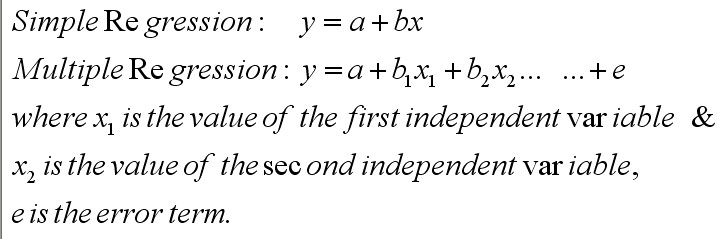
[The
error term is there because it highlights the fact that a proportion of the variance
in the dependent variable; y, is unexplained by the regression equation.
In most cases, and certainly when making predictions for values of y', the error
term is ignored.
We
are now looking towards predicting a value for y ( that is:y') using data from
two or more different
independent variables (x1 and
x2). We will still need to calculate
'a', the interception point on the Y
axis and 'b1' and (b2),
the regression coefficients.
Multiple
regression examines the relationship between several independent variables (not
necessarily restricted to just two or three ) and one dependent variable.
As with simple regression, the data
must be at least normally distributed and metric.
There
are several approaches that can be taken here; one is simultaneous
multiple regression where all the independent
variables are entered into the equation simultaneously. There is
also stepwise multiple regression
where each independent variable is dealt with one at a time.
Although
SPSS can easily carry out both procedures, the interpretation of the latter is
more difficult and so we will only concentrate on simultaneous
multiple regression here.
There
is no point in adding a second independent variable to the work unless the situation
is that the second one is going to add some unique contribution to our understanding
of the behaviour of the dependent variable. The extra independent variable must
add information about the behaviour of y that the first one cannot. It
is important that both (all) independent variables only relate to the dependent
variable and not directly to each other.
We
must therefore ask the following questions:
"
Does the addition of more independent variables improve the accuracy of our predictions"?
"
Is one of the variables more (or less) influential than the other"
 In a customer survey, the 'ME & YOU'
garden centre chain (18 stores) wanted to know if rainfall kept customers away
and thereby possibly affecting plant sales. Also, did the age of the customers
have any affect upon sales figures? Only rainy days were included in the survey.
The mean age of approximately 56 customers per store was used.
In a customer survey, the 'ME & YOU'
garden centre chain (18 stores) wanted to know if rainfall kept customers away
and thereby possibly affecting plant sales. Also, did the age of the customers
have any affect upon sales figures? Only rainy days were included in the survey.
The mean age of approximately 56 customers per store was used.
Q.
Would it have been better for the company to compare 'rainy day' sales with 'non-rainy
day' sales?
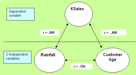
So
'rainfall' and 'customer average age' are the 2 independent variables and we have
one dependent variable....'£sales in 24 hours'
Use:
SPsmAex12 Supermkrain
(You must study carefully how this data set has been entered)
We
may well surmise that both rainfall and customer age will affect final
sales.
We have 3 variables x 18 cases to handle.
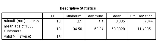
To
get a 'picture' of any possible relationships, always begin by using SPSS to generate
the usual 'descriptives output (to give us the mean values of any of the variables)
and by plotting the two graphs....
Go
to graphs , 'Scattergraphs', 'simple' and click 'OK'.
Put 'Rainfall' (and
then 'Customer age' ) on the 'X' axis and run both against '£ sales' on
the Y axis.......
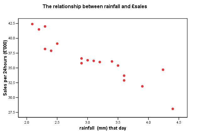
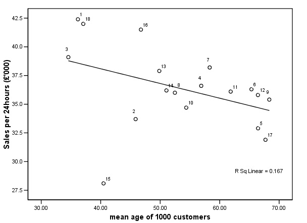
So
it appears that we have a negative correlation between 'rainfall' and '£sales'
and
also between 'customer age' and sales...... 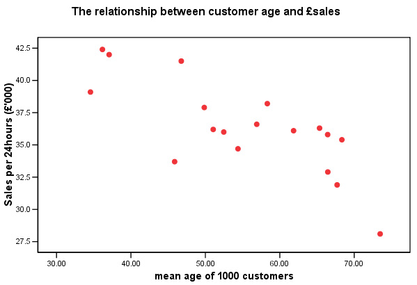
but we do not know whether one of these factors is having
a greater or lesser effect on the outcome than the other. The
next step then, is to calculate and compare the 3 possible correlations.
Q.
Should we be carrying out a correlation test between the
two independent variables? A. No!.
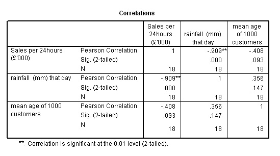
Firstly, go to 'analyse', 'correlate' ,'bivariate'
and transfer all 3 variables
Here
is the output>>>>
*Remember
that if you highlight an output frame and place the cursor over an SPSS Sig-value
reading .ooo, and double left-click the mouse, you
can obtain the exact p-value.
The
above chart could be summarised as....
Just
as we suspected, there is a strong negative correlation between '£sales'
and 'rainfall' (R= -.909) and a weaker result for 'Customer age' and '£sales'.
| Caution
! We
have also found a spurious relationship between the two independent variables:'rainfall'
and 'age of customer'. These variables could not both be independent if one was
able to influence the other. This is instructive because it shows how easy it
is to create illusions and false assumptions with numerical data if you are unwary. |
|
"The
more rain; the less £ sales" (r = -.909)(strong negative correlation) "The
older the customers, the less sales" (r = -.408)(medium negative correlation) |
SPSS:
Note
that by ticking 'casewise diagnostics' from the 'statistics' button from the Linear
regression window; the same output
can be obtained.
Now
go to 'Analyse', 'Regression', 'Linear' and transfer '£sales' to the dependent
variable box. Transfer 'rainfall' and 'customer age' to the independent variable
box.
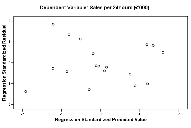
Click 'Plot' and place 'ZRESID' in the Y box and 'ZPRED' in the X box.
Click
'OK'
The
requested scatterplot should appear last in the output but look at it first.....
In
this case it shows little obvious pattern. If any systematic patterning between
predicted values and residuals were indicated, it would suggest possible
violations of the assumptions of linearity. The chart below shows no patterning
and this confirms that the assumptions about the suitability of the data for this
type of analysis have been met and that we can continue...
The
next output to study (see below) is the 'Model Summary'. The adjusted R square
value shown in the output is the proportion of variance accounted for by regression,
this value may be expressed
as a % i.e. 81.3%. We
will use this information later to decide whether or not the utilisation of the
second independent variable has improved our predictive ability in the analysis
or not.
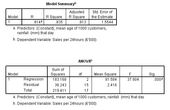
The
ANOVA analysis shows that the regression is highly significant (P<0.001).
We
deal with ANOVA more fully in Focus 13.
Next
we can work out the equation for the regression line and check it against the
charts we
produced earlier. Our two regression co-efficients are -4.461 and
-0.030 respectively.
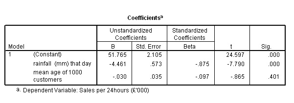
The
Standardised beta coefficients are also very useful
as they indicate which of the two independent variables influences the dependent
variable the most. Now all the variables are standardised and expressed as z-scores.
This represents the number of standard deviation changes caused to the dependent
variable(£sales) by the change of one s.d. to each /any of the independent
variables. In our case it is rainfall levels with
a Standardised beta coefficient of -.875 as compared to the
age value of -.097 that makes the greatest contribution to the variability
in the dependent variable.
The Regression Equation
We derive the multiple regression equation using column B from the coefficients
output (shown earlier)....
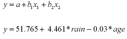
and
therefore y mean(£sales) = 51.765 - [(4.461*rainfall
mean) - ( 0.03*customer age mean)] i.e.
y mean = 51.765 - [( 4.461*3.085) - (0.03* 53.333)] =
51.765 - [13.762 - 1.599] = 39.603
(39.60) ------------------------------------------------------------------------------------------------------------------------------------ Let
us use the formula to examine the 3rd , 10th and 12th cases
from the original dataset. 3rd:
where the rainfall was 2.5mm and the mean customer age was 34.56 y'
= 51.765 - [( 4.461* 2.5) - (0.03*34.56) = 39.58
(£39,580.00) Our predicted
value for y' is 39.58 and the actual value was 39.1; a difference
= (-0.48) 10th:
where the rainfall was 4.2mm and the mean customer age was 54.38 y'
= 51.765 - [(4.461*4.2) - (0.03*54.38 )] = 51.765
- (18.736 - 1.631) = 31.40....(£31,400.00) Our
predicted value for y' is 31.4 and the actual value was 34.7
The difference = (+3.3) reflects
the 'distance' the observed value is away from the lines of best fit....on the
Y axis. Note
how the second independent variable has an appreciably lesser effect upon the
result than the first independent variable seems to have. 12th:
Predicted y' = 36.8, actual = 35.8, difference
= (-1.0)
Look at the first of the two regression lines below, case 3 is close to the line
in both charts. In
case 10, the stronger influence (rainfall) place the value well above the line.
The weaker of the two influences places it just below the line but here, the influence
is too small to make a difference. Case
12 is a uniform distance from the line (one case just above and one just below)
in the two charts but the former has greater influence on the outcome........ 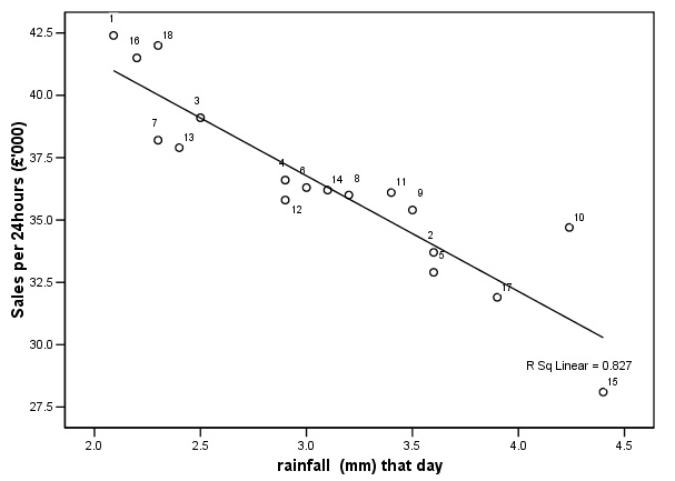
& 
The
difference between 'Predicted' and 'Actual' is referred to as before; as the 'Residual'. Task:
Comment on case 15. Would you suggest removing it from the analysis and if so,
why? Can you offer any possible reasons for such an anomalous result for this
particular garden centre?. |
We noticed that the multiple correlation coefficient
shown in the Model summary above was:
R = .914 and the adjusted R square
value: .813 (81.3%).
So
utilising a second independent variable (age) has, (in this instance) marginally
reduced the predictive power of the regression from (1) 81.6% and (2) 11.4%(when
carried out individually) to.... 81.3% overall and it was
therefore not worth adding the second independent variable.
In
summary we can say that both factors have a significant effect (p<0.01) upon
sales, that there is a strong negative correlation between 'rainfall' and '£sales'
and a medium negative correlation between 'age of customers' and '£sales'.
Furthermore,
because we carried out a multiple regression analysis instead of two simple linear
regressions, we
can add that 'rainfall' has a far greater influence on sales than 'age' does.
Predicting
values for y'
We
can also now predict what the sales should be if we are given the 'rainfall' level
and the 'mean age of customers' figure. The same
rules concerning the validity of interpolation and the risks associated with extrapolation
as discussed in Focus 11
E.g:
Imagine that we have a situation where there was half the rainfall but a similar
'age' profile for the customers (the variable with the lesser influence) than
cited in case 10 above(4.2 mm and 54.38 years)...would
you expect the sales to increase or decrease?
So:
'rainfall' = 2.1mm, 'mean age of customers' = 56.0
y'
= 51.765 - [(4.461*2.1) + (0.03*56)] = £40,717....a
large increase!
Task:
Use 'rainfall' = 3.2mm and 'mean customer age' of 59.5 to predict sales that day.
A four-variable model
In
the above example we used one one dependent variable and two independent ones.
In this example, we will use one dependent variable (sales
again!!) and three independent ones.
 A high street gaming store sells DVD's and CD's. The store manager keeps accurate
monthly records of their sales figures. He knows that the unit 'buying-in' price
dictates his selling price and that in turn probably determines overall sales
for the month. However, he has suggested that the amount spent on promotion and
the general levels of economic activity in the market place may also affect sales.
How do these three variables affect overall sales? In this example, we will attempt
to unravel the mystery!
A high street gaming store sells DVD's and CD's. The store manager keeps accurate
monthly records of their sales figures. He knows that the unit 'buying-in' price
dictates his selling price and that in turn probably determines overall sales
for the month. However, he has suggested that the amount spent on promotion and
the general levels of economic activity in the market place may also affect sales.
How do these three variables affect overall sales? In this example, we will attempt
to unravel the mystery!
You must use:
SPex63
DVD games
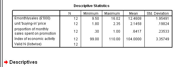
Firstly,
go to 'analyse', 'descriptive statistics','descriptives' transfer al four variables
and click 'ok'
Note
the mean values for the four variables...
Next,
go to 'Analyze', 'correlate' ,'bivariate' and transfer all 4 variables. Here
is part of the output>>>>

The
chart above shows a fairly strong positive correlation between '£sales'
and 'unit price', a weaker positive relationship between '£sales' and 'promotional
effort' and an even weaker positive relationship with 'economic activity'
Task:
Produce 3 scattergraphs to illustrate the above statement.
Now
carry out the linear regression analysis just as before except this time, transfer
all 3 independent variables instead of just two....
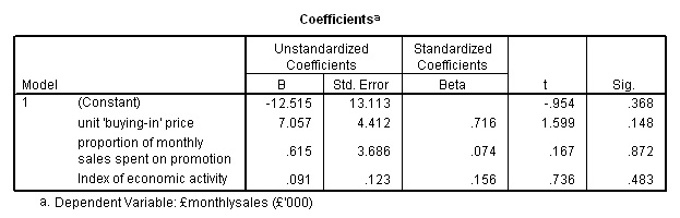
The
formula for the regression line is:
y =
-12.515 + 7.057[buying price] + 0.615 [promo
effort] + 0.091 [econ activity]
y[mean] = -12.515 + (7.057*2.145)
+ (0.615*0.642) + (0.091*104)
= 12.49
correct!
So
now we can make predictions for a monthly value for y; given values for the three
independent variables.
E.g. The buying
price is 2.10, the promotional effort is 0.85 and the economic activity level
is 105
y' = -12.515 + (7.057* 2.1) + (0.615*0.85)
+ (0.091*105)
= -12.515 + 14.820 + 0.523
+ 9.555 = 12.383 (£12,383)
Note
that although there was a good correlation between 'promotional effort' and '£sales'
(.706); the Standardised Beta coefficient was very low (.074) and if you look
back at the worked values in the regression equation you will see that the contribution
made by this variable is quite small.
So
the manager was right by deducing that the unit buying price( and therefore; selling
price) that has the greatest effect upon sales followed by economic activity and
least of all by promotional effort.
Moving
on to thinking in three dimensions!
In
multiple regression work, we have been looking at the comparative influence of
n different variables upon the one dependent variable under investigation. Until
this Focus page, we have nevertheless, worked in just two dimensions; X and Y.
In later Focus pages we will look at the relationships that might exist between
numerous variables and for this we must think in 3D!
In
the previous example, we looked at the relationships between three
variables, in order to see how they interact with each other, we would need to
draw three scattergraphs: AB, AC and BC. It is possible to use SPSS to plot a
3D chart so that all three variables can be viewed simultaneously. This will help
to 'visualise' how the variables are behaving with respect to each other.
Try
to imagine that the points are floating 'magnets' and the three axes are fixed
magnets that are continually attracting or repelling the individual points proportionately
to the strength of the magnets.
Go
to 'Graphs', 'Scatter', '3D' and 'define'
Transfer
'£sales' to the Y axis, 'Rainfall' to the X axis and 'Age of customers'
to the Z axis. Click 'OK'.....
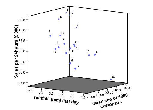
Task:
Try to describe how much 'top to bottom' (XY) variation you can detect in the
above chart and then how much 'front to back' (ZY) variation there is. Remember
that each of the points in space represent the values from just one garden centre
and they have all produced a slightly different result from each other. We could
perhaps suggest that each 'point in space' characterised that particular garden
centre. These sets of characteristics are often called 'signatures' and we will
return to this concept in a later Focus.

Go
back to 'quick view' contents
Go
back to Focus 11
Go on to Focus
13 (ANOVA)