[Focus 13]A brief introduction to ANOVA's....(1)
Regression ANOVA's |
You will remember that calculating the standard deviation is a useful way of measuring the variation within a sample of data and for then making comparisons between other data sets. Variance is always the square of the standard deviation.
There
are a number of definitions used to describe ANOVA's but in essence they form
a suite of tests used when we want to assess the differences
between the means of several samples
and to assess whether they
have come from a single population. The logic
used is similar to that applied to independent samples
t-tests
For all ANOVA tests; data should be at least on the Interval scale* and normally distributed but there are a number of other limitations and assumptions we must first consider below.... (See also Levene's test for homogeneity below)
*Note however, that we can use the Kruskal - Wallis one-way analysis of variance for ranked (ordinal data).
ANOVA'S come in at least 5 main designs depending upon:
a) the type of survey or research design being used
b) the comparisons that are being made.
We must define whether the groups under investigation are:
|
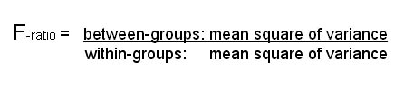
The idea of the F-ratio is crucial to understanding how ANOVA works. The rationale is to check whether there is more variation ( i.e. measured variance) between the samples than within them. We will be calculating that ratio (known as the F-ratio) by using the mean squares (MS) of the 'between-groups' variance as the numerator and the 'within-groups' variance as the denominator.
We began to explore the idea of variation 'between' and 'within' back in Focus 4....
 Imagine that the Britmax factories in Bournemouth
and Reading were to monitor the output per employee per week for a number of months.
Firstly we could examine the factories individually and we would see that the
outputs vary from week to week (blue arrows). Then we could compare the variation
shown between the two factories (green arrows).
Imagine that the Britmax factories in Bournemouth
and Reading were to monitor the output per employee per week for a number of months.
Firstly we could examine the factories individually and we would see that the
outputs vary from week to week (blue arrows). Then we could compare the variation
shown between the two factories (green arrows).
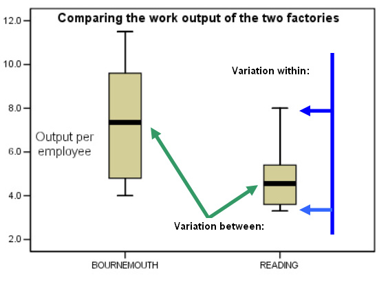
[Cautionary note: the 'Boxplot' is not an ideal method of illustrating the idea of 'within' and 'between' because they are really illustrating 'range', interquartile range' and medians. Nevertheless it should convey to you the important idea that 'variation' may be thought of as existing in two forms].
Remember:
| Important Rule.... " The larger the ratio indicated by the 'between' and 'within' variations, then the more likely it is that the two means are significantly different". |
Let
us imagine two cases: those where the 'between-groups' mean square figure is 12
and then when it is 6.
In both cases let the 'within-groups' figure remain
at 3....
If the 'between-groups' figure is a lot larger than
the 'within-group' figure, the F-ratio is going to be a large figure e.g. 12
÷ 3 = 4 but if the variation 'between-groups'
is small e.g. 6 ÷
3 = 2.... then the F-ratio
will be smaller also.
| Between
groups | Within
groups | F-ratio |
| 12 |
3 |
4 |
|
6 |
3 |
2 |
| The
greater the value of F the less likely it is that the samples come from the same population. |
Once again, you need to be sure that your data is Normally distributed to begin with.
We can now use tables to check up on the critical values for F that will allow us to determine the level of statistical significance that the F-ratio value obtained. Remember that a prerequisite of any significance test is that a null hypothesis and an alternative hypothesis must always be constructed.
As
usual, firstly the 5% level and then the 1% level is checked. Remember also that
SPSS allows
you to take the probability of F directly from the output
so you are not restricted to only quoting
a 5% or 1% value.
If using tables; remember that the F-value(calc) must exceed the critical value(tab) in order to achieve significance at that level.
Because there are a number of prescribed steps before the F-ratio and the P value can be calculated, there is a strict ANOVA summary table format which you should learn to recognise and always use.
| Source of data | Sum of squares | d.f. | Mean Squares | F-ratio | P value |
| Between Groups | |||||
| Within Groups |
We can !! The problem is that if we had three groups to compare, A, B, and C we would have to do an AB, AC and a BC t-test. This is perhaps not unreasonable but if we had say 5 categories we would have to do 10!
The other problem
is that the more t-tests we do in a set (especially once we reach 7 categories
= 21 tests) , the more likely we are to obtain a statistically significant result
by chance alone. If we have set our critical probability at 0.05 we are likely
to reject the null hypothesis at least once for every
20 t-tests we carry
out. This would be a type 1 error.
Fortunately, if we do just one ANOVA, we can simultaneously compare all our means and the overall probability of incurring a Type 1 error stays the same.
You should also read the section on Tukey's test below...
Before dealing directly with one-factor ANOVA's, it will be useful to go back and consider our regression graphs once more where just two variables are involved (Focus 11). Regression ANOVA's look at the strength of the relationship between two variables i.e. just one factor is 'in play'.
Regression ANOVA's are essentially dealing with 2 factor variables and a single dependent variable. We have stated above that a very useful way to compare any two (or more) groups is to look at the variance ratios and to produce a value for the F-ratio.
Study the chart below and make sure that you can see why there are three elements to the variation displayed. There are three particular values involved:
The mean value of y is 3.4 and the pale blue line indicates this position. We are interested to know how that variation (of 2.4) is made up and the chart below explains this.
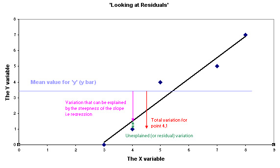
ANOVA looks at the ratios of the explained (or 'the effect') variation (pink arrow) to the unexplained (or 'the error / residual') variation (green arrow). When y = 1; variation away from the mean value for 'y' of 3.4:
2.0 : 0.4 gives a ratio of 'explained' to 'unexplained' of 5 : 1. |
Naturally this ratio will not apply to the other points on the graph as they are all at different distances from the 'line of best fit' and the horizontal mean of Y. So we need to explore the variation that exists between the points as well as the variation within or unique to each individual point.
We must always start with a null hypothesis:
"The variation in 'y' is not accounted for by the variation in 'x' "
and the alternative hypothesis:
"The variation in 'y' is accounted for by the variation in 'x' "
The first task is to square all true variation values (for each point) in order to make them positive.
| Sum of squares (SS) calculations (Regression ANOVA): The order of working follows the simple rule (refer to the arrows in the previous chart): if A = B + C then, C = A - B Thus: SS(total) = SS(explained / regression) + SS (unexplained / residual) and SS(resid) = SS(tot) - SS(regres) We calculate A first, then B, take B from A to give C. The respective formulae for SS (total) and SS (regression) are given below.... |
Manual method:
Once
again, the formulae involved are lengthy rather than complex and so it is wise
to begin with a
full tabulation of all that is needed before attempting any
calculations because it is easy to muddle the figures.
Although not essential to the calculation, remember that a plot of the data (using Excel in this case) may help to clarify things....
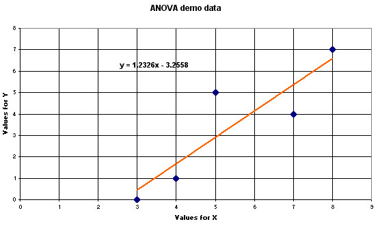
Study the various distances that each point is away from the regression line (only with regards to the 'Y' axis). Note also that, as with any 'line of best fit', explained variations (within each point), when all added together will equal zero.
Check....
| "when
'x' = " | 'y'
(actual) | 'y'
(on regression line) | 'y'
difference | above
/ below (+/-) |
| 3 |
0 |
0.442 |
0.442 |
- |
| 4 |
1 |
1.675 |
0.675 |
- |
| 5 |
5 |
2.907 |
2.093 |
+ |
| 7 |
4 |
5.372 |
1.372 |
- |
| 8 |
7 |
6.605 |
0.395 |
+ |
| |
|
|
|
total + =2.488 total - =2.489 |
The question is: How much of the variation (fourth column above) shown in 'y' can be accounted for by the variation in 'x'
First find: SS (total)..... and then SS (regression), take one from the other to give SS (residual).
You also need to record: n = 5, mean of 'x' = 5.4 and the mean of 'y' = 3.4
| 'x' |
'x' squared | 'y' |
'y' squared | 'xy' | |
|
|
|
|
|
| |
| 3 |
9 |
0 |
0 |
0 | |
| 4 |
16 |
1 |
1 |
4 | |
| 5 |
25 |
5 |
25 |
25 | |
| 7 |
49 |
4 |
16 |
28 | |
| 8 |
64 |
7 |
49 |
56 | |
| SUM (sigma) | 27 |
163 |
17 |
91 |
113 |
| Means | 5.4 | 3.4 | |||
& sigma'xy'
|
& = 729 | &
= 289 |
So this is all the information needed to undertake a one factor ANOVA other than the formulae themselves:
So: SS(residual) = 33.2 - 26.13 = 7.07.
The final stage is to fill out the ANOVA table which always follows the convention described earlier:
| SS |
df | Mean Square (MS) | F (the test statistic) | P | |
| Regression ('the effect') | *** | 1 | SS(regression) ÷1 | MS(regression) ÷ MS (residual) | |
| Residual ('the error') | *** | difference between the Regression d.f. and the total d.f. |
SS (residual) ÷ <<< that diff | ||
| Total | *** | n -1 | |||
In our case (where n = 5) this becomes:
| SS |
df |
MS |
F-ratio |
P | |
| Regression |
26.13 |
1 |
26.13 |
11.088 |
* |
| Residual |
7.07 |
3 |
2.357 |
| |
| Total |
33.2 |
4 |
| ||
So our final result gives n F-ratio(calc) of 11.088
| Clarification of the above
calculations: 26.13 ÷ 1 = 26.13 7.07 ÷ 3 = 2.357 26.13 ÷ 2.357 = 11.088 |
* We now look up in the
F values table for Regression df: 1 and Residual df: 3 and we find a
figure
10.1 for P = 0.05 and another figure of 34.1
for P =0.01
Our test result (11.088) is higher than 10.1 and so we cannot accept the null hypothesis at the P(0.05) level but the situation is different at the P (0.01) level as we have not exceeded 34.1.
So we can say that a statistically significant amount (P(0.05)) of the variation in 'y' is accounted for by the variation in 'x'.
Note
that the P value is given to an exact value (Sig : .045) showing that we have
exceeded the critical
value for P(0.05)but not any greater level of significance.
Note also that SPSS does not list what that critical value is (it is not necessary).
To discover what the critical value is, we would still have to use tables.
From the manual working above you will recall that for P(0.05), it was 10.1.
We also have the necessary values to complete the regression formula for this particular line:
y = - 3.256 + 1.233x or re-arranged as y = 1.233x - 3.256
As
a check, we know that any 'line of best fit' must pass through the mean of 'x'
and the mean of 'y'.
The mean of all the 'x' values is 5.4 so substitute
this value in the formula.
y(mean) = 6.658 - 3.256 = 3.402, the mean of 'y' was also found (from the data set) to be 17÷ 5 = 3.4
Correct!
Let us next carry out a regression ANOVA fully using SPSS...
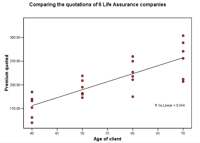
 The Daily Mail, 'money page' has carried out a comparison
survey of Life Assurance premiums. They asked 6 leading providers to give quotations
for healthy males aged 40, 50, 60 and 70, all living in the same location and
with similar jobs. How can we best compare the quotations?
The Daily Mail, 'money page' has carried out a comparison
survey of Life Assurance premiums. They asked 6 leading providers to give quotations
for healthy males aged 40, 50, 60 and 70, all living in the same location and
with similar jobs. How can we best compare the quotations?
We can quickly produce a 'line of best fit' but just how valid is the inference? You might say that if all the points fall close to the line then this will give us a good indication (and this is true) but it is not very scientific. ANOVA will give a more precise result.
Task:Construct your null and alternative hypotheses.
The data set is:SPex59 Life Assurance ANOVA
Open SPSS in the usual way, the two variables are 'age' and '£quoted' , produce a simple scattergraph and then superimpose the regression line...
Note that we are treating all the quotations as though they belong to one group.
Q. What effect do you think this might have on the result?
Hint: A one-way ANOVA would be even more accurate (as described later).
Go to 'Analyse', 'Regression', 'Linear' & tick 'Statistics' (this gives the descriptives i.e. means and s.d)
The output involves 5 frames but here are the two most important that you should have generated....
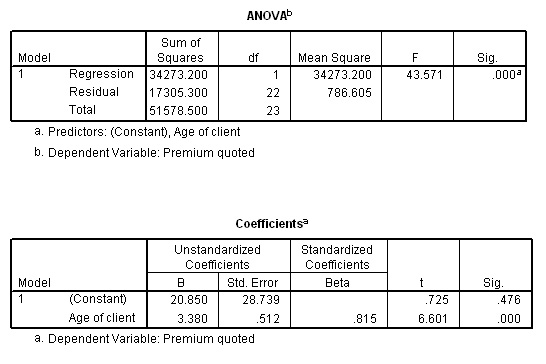
The formula for the line is: y = 20.85 + 3.38x
Task: Check that this is correct (hint: you will need to obtain the mean of x and y )
Task:The F- ratio is shown to be 43.571, how would you find the critical values for P at both 5% and 1%.
Explain the SPSS output for P(sig)
Q. Why can we not simply use an Independent samples t-test on this dataset?
If we now carry out the alternative one-way ANOVA test on the same data set ....
Open the dataset as above: Go to 'Analyse', 'Compare Means', 'One-way ANOVA'.
Transfer 'premium quoted' to the dependent box and 'age of client' to the factor box
Click
'options' and tick the 'Descriptives' and 'means plot' boxes.... also tick the
'Homogeneity-of-variance' box (see note
below concerning the Levene statistic)
Click 'continue' and then 'OK'.....
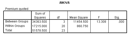
We get the same result in terms of the level of significance but a much lower (more stringent) F-value of 13.308. This is because we are now being more precise and treating the data as 4 separate (age) groups rather than one large one as we were with Regression ANOVA.
Caution! the d.f. values are now calculated quite differently.When carrying out the regression ANOVA we had 4 degrees of freedom recorded. We were in effect, treating all 24 quotations as applying to one group....'clients', this is not strictly true because the clients were from 4 quite different age groups. It is important that the changed calculation method regarding degrees of freedom for ANOVA calculations are clearly understood.... 1) Start with d.f. Total. We had 24 quotations. So to reach the correct values for the mean / standard deviation 23 can vary but once they become fixed, the last one (24th) cannot. Therefore: 23 2) Between Groups. Here is where the big difference lies, we now have an additional capability to deal with i.e. 'between groups' variation. There were 4 groups (see graph above). These must also add up to the grand total of 4, so as soon as three become fixed the last one cannot vary i.e. n - 1d.f. and in this case that means 3. Remember, in the regression ANOVA we placed all the values in one group. Therefore now: 3 3) Within groups. This always has to be the difference between the two i.e. 20. Or you may prefer to think of it as 6 scores per group >>> yields 5 d.f. and as there are 4 groups....5 x 4 = 20. Conclusion: 23(total d.f) = 3(between) + 20(within)
|
 Multigym International have many fitness clubs throughout the UK but 110
branches are situated in busy city centres and cater for lunchtime users mainly.
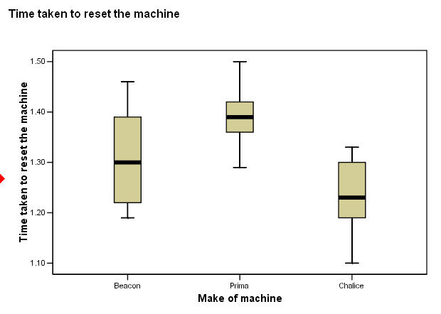
They are currently testing 3 three new makes of 'executive' rowing machines ('Beacon','Prima',
and 'Chalice') to see if there is any real differences between the three. Before
buying these very expensive machines it is important to know which allows the
fastest 'turnaround' time because this is a crucial element in the selection process.
Timers were attached to each machine and the results analysed. Of course, there
may be no discernible differences between the three.
Multigym International have many fitness clubs throughout the UK but 110
branches are situated in busy city centres and cater for lunchtime users mainly.
They are currently testing 3 three new makes of 'executive' rowing machines ('Beacon','Prima',
and 'Chalice') to see if there is any real differences between the three. Before
buying these very expensive machines it is important to know which allows the
fastest 'turnaround' time because this is a crucial element in the selection process.
Timers were attached to each machine and the results analysed. Of course, there
may be no discernible differences between the three.
6 branches were to chosen to participate and each had each of the three machines installed in turn.Thus there are 18 results to consider...
Here is the basic data set... SPex 75 Multigym
(figures in brackets are that value squared)
| 'Turnaround' time ( in minutes) >>> | 'Beacon' |
'Prima' |
'Chalice' | |
| Branch | ||||
| 1 |
1.27 (1.613) | 1.50 (2.250) | 1.10 (1.210) | |
| 2 |
1.33 (1.769) | 1.41 (1.988) | 1.19 (1.416) | |
| 3 |
1.46 (2.132) | 1.37 (1.877) | 1.27 (1.613) | |
| 4 |
1.39 (1.932) | 1.36 (1.850) | 1.33 (1.769) | |
| 5 |
1.22 (1.488) | 1.42 (2.016) | 1.30 (1.690) | |
| 6 |
1.19 (1.416) | 1.29 (1.664) | 1.19 (1.416) | |
| Sum (mins) | ...7.86 (61.780) |
...8.35 (69.723) |
...7.38 (54.464) | 23.59 (556.488) |
|
Mean (mins) | ...1.31 |
...1.39 |
...1.23 | 1.311 |
These
results present the company with a dilemma because the mean turnaround times seem
so similar but can we be sure?
Can we say that statistically, there is no
real difference between the three or is there a significant difference?
Task: Construct your own Ho and H1.
The calculations should be done manually to follow the progress of the calculation:
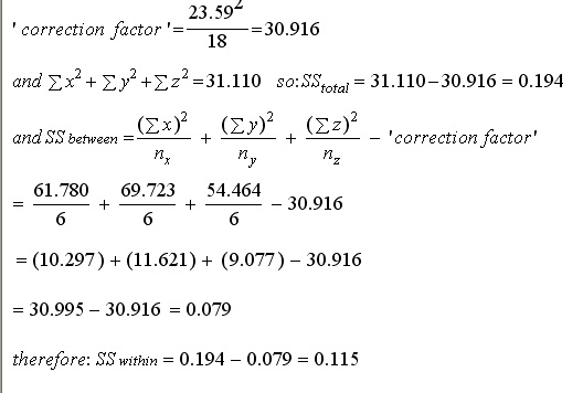
Grand total time: 23.59 mins.......grand mean (divide by 18) = 1.311 mins
Now calculate the square of each of the 18 values (already shown in brackets above) and sum them. 1.613 + 1.769 + 2.132 etc etc =.... this gives a total of 31.110
Thus SS (total) would appear to be 31.110 but we will first need to incorporate a correction factor (see second box below)..
Assessing the variation:Remember: (Total variation) = (Within Group) variation + (Between group) variation So Sum of squares (SS) calculations (One-Factor Independent groups ANOVA): SS(total) = SS(between groups) + SS (within groups) and SS(within) = SS(tot) - SS(between) The respective calculations for SS (total) and SS (between) are given below. As with regression ANOVA; we have to calculate the 3 SS values strictly in the correct order: (1) SS total.......(2) SS between....... (3) SS within |
Now we need to find the final expression for SS (total) and this is explained below:
| To obtain the true SS (total), as explained, we need first, the sum of the squares of all the individual values (31.110). However: it is necessary to deduct a second expression; which is the Grand Total squared divided by the total number of values in all samples. This term is sometimes referred to as the 'correction factor'....
= 23.59 squared (= 556.488, then divided by 18 = 30.916). So
the CF = 30.196. We will also need this expression to calculate the SS (between) value. |
At this point we can say that the sum of squares (between) + the sum of squares (within) must add up to 0.194
Now for the SS (between-groups)
Square the sum of each group and then divide the answer by the n for that group...
'Beacon' .......7.86 squared = 61.780 divided by 6 = 10.2966
'Prima' ...........8.35 squared = 69.723 divided by 6 = 11.6205
'Chalice' ........7.38 squared = 54.464 divided by 6 = 9.0774
all summed = 30.9945 (i.e 30.995)
Once again, subtract the (already calculated) correction factor (30.916) = 0.079
Finally, the SS(within-groups) must be the difference i.e. 0.194 - 0.079 = 0.115
Let us follow this same method in a mathematical layout...
We now have all the details necessary to construct and complete the standard ANOVA table....
n
=18
|
| SS |
d.f. |
MS |
F-ratio |
P |
| Between groups | 0.079 |
2 |
0.0395 |
5.15 |
<0.05 |
| Within groups | 0.115 |
15 |
0.00767 | ||
| Total |
0.194 |
17 | |||
From tables (table D7, p222 in Wheater & Cook) we find that P(0.05)(d.f.2,15) the critical value for F is 3.68 and at P(0.01)(d.f.2, 15) it is 6.36
Remember, results are significant if our calculated value (5.15) is greater than the tabulated value. Compare your conclusion to that shown in the SPSS output below....
Task: Write down the conclusion for these results and relate them back to H1 and H0.
Enter the names and labels in the usual way and then enter the data or use: SPex 75 Multigym
It is important to check for outliers before conducting the analysis, so........ Go to 'Graphs', 'Boxplot', 'Simple'. Put Radio button in 'Summaries for Groups of cases' Define..... Variable as 'time', Category Axis as 'make ofmachine' and label cases by 'club number'...
You can see that whilst there is a clear difference between the results obtained for each machine, there are no outliers to worry about and so the analysis can go forward..... Can you remember how to interpret a Boxplot? See Focus 3b |
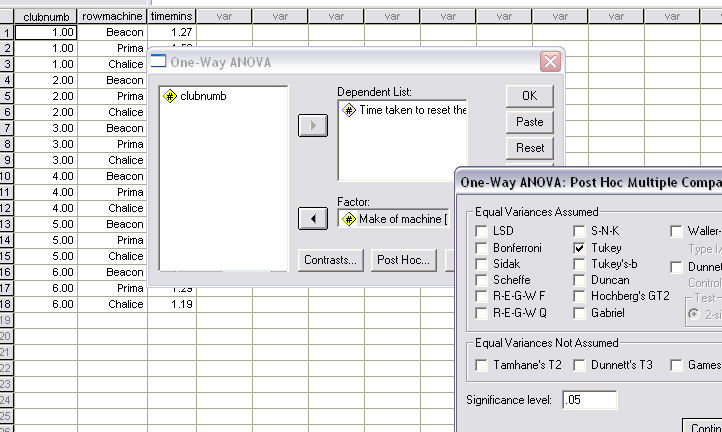
Now go to 'Analyse', 'Compare Means', 'One-way ANOVA'.
Transfer 'time ' to the dependent box and 'make of machine' to the factor box
Click
'options' and tick the 'Descriptives' and 'means plot' boxes....
also tick
the 'Homogeneity-of-variance' box (see note below concerning the Levene statistic)
Click 'continue' and then 'OK'.....
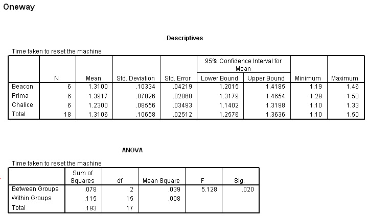
The difference in the F-ratio between the manual (5.15) and SPSS (5.128) methods is simply a rounding difference.
Once again, SPSS gives a direct P value (.020) for the significance of our F-statistic. Compare this with the result obtained via the manual method.
Task: Indicate which machine is 13% faster than which other machine.
Q. Which machine would you advise the Company to include in their buying policy?
Homogeneity could be defined as "the level of 'equality' between the samples".
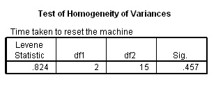
The Levene test examines whether the variance (variation) of values for the groups is generally the same. It does not have anything to do with disparity of sample size. In SPSS the outcome of the test will determine if there is or is not evidence of homogeneity or the opposite state; heterogeneity. The P-value for the Levene statistic is significant if the output shows it to be less than 0.05 and in those circumstances; equal variance must not be assumed.
Here is the output from the multigym example, the Levene statistic is .824 and is therefore not significant, so equal variance can be assumed....
| Alternatively, the two-category Chi square test can be used to test for homogeneity. H0 would state that there was no bias and H1(the alternative hypothesis) would state that there was bias present in the data set. |
Post hoc tests are carried out once the issue of significance has been established. After all, there is little point in checking on the 'fine tuning' of a significance output if the result is not significant in the first place! If there is no significant difference detected, then that is the end of the analysis.
The
test is designed to make adjustments that help to lower the risk of making a Type
1 error.
(Type
1 and 2 errors are important and are fully explained in Focus
4)
If there are only two means involved and the results indicate a significant difference between the two; then the answer is simple, "the larger mean is significantly larger than the smaller one "!
Unfortunately, we cannot say this when there are 3 or more means involved. There will be several possible scenarios and to determine exactly where the differences lie, we need to carry out a comparison test.
Tukey's test assumes equal variance. The test will compare all possible combinations of pairs of means:
| number
of means involved |
number of necessary pair-comparisons |
| 2 |
1 |
| 3 |
3 |
| 4 |
6 |
| 5 |
10 |
| 6 |
15 |
Be aware however, that the more tests we do,the more likely we are to falsely reject a null hypothesis and claim a significant difference when in fact there is none....a Type 1 error . If we do nothing (that is leave the calculation at the point where we have concluded an overall significant difference, we are in danger of committing a Type 2 error.
Tukey's test is often referred to as yielding the HSD (honestly significant difference) test and is a compromise between the two risks outlined above.
Let us return to the
three makes of rowing machines ....
Go back to the SPSS menu and carry out the procedure as before but this time also click on the 'post hoc' box and select the 'Tukey test'...
and here is the output...
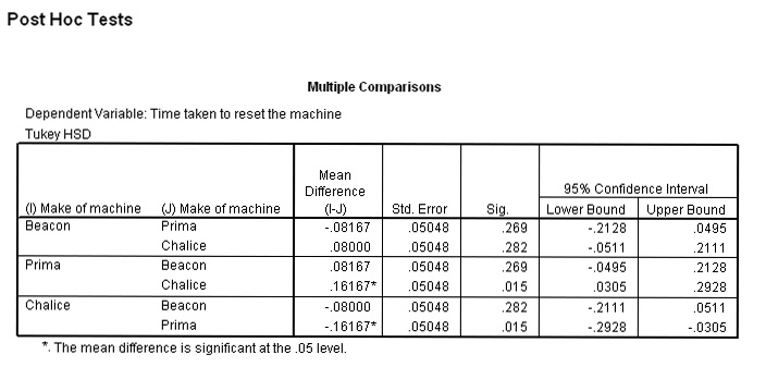
This
chart shows that there is a significant difference
between the 'Prima' and 'Chalice' machines
P= (0.015), but no other comparisons
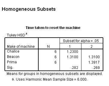
of the means showed a significant difference. This is made clearer in the chart
below; each machine has been slotted into a group with any of its homogeneous
partners and again it can be seen that because 'Chalice' and 'Prima' have been
found to be significantly different (at least as far as 'set up time' is concerned),
they have been placed in separate subsets by SPSS.....
Q. Are these findings borne out by the boxplot we produced earlier?
Task: Carry out the next analysis yourself....
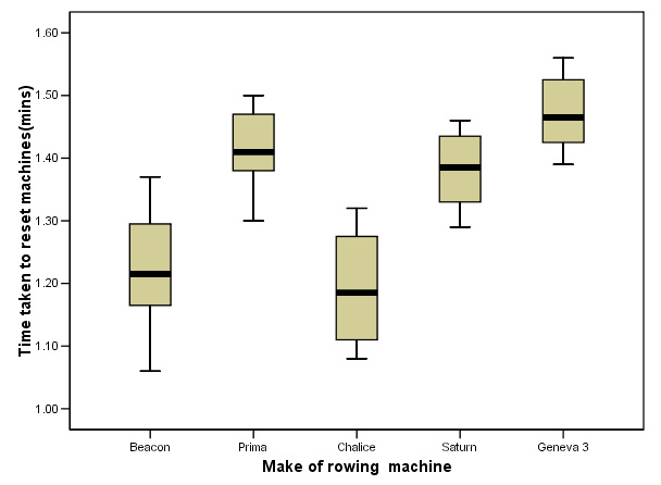
The trial was conducted again the following year on a slightly larger scale and
now 5 machines were
tested including two new computerised 'hi tech' versions; 'Saturn' and 'Geneva
3'.
Use:SPex 76 Multigym 2 to carry this analysis >>>>
Remember to construct an H0 and H1 before you begin.
Task: produce your own boxplot as below........
Task: Carry out a One-way ANOVA and the post hoc (Tukey's) test
Task: Explain your results in such a way as to be comprehensible in a Powerpoint presentation to a group of branch managers.
Britmax are evaluating three new robot welding machines from three different manufactures
for use in constructing their bike frames. The assembly team was asked to turn
out 6 frames from each machine and to record exactly the time it took to complete
each frame.
The results are recorded in SPex62 ANOVA bike frames. After carrying out the work, the results are analysed using a one-way ANOVA test (as above). There is found to be a significant difference (P-value 0.007) between the three machines in terms of construction times.
Remember to construct an H0 and H1 before you begin.
Q. Which is the fastest and which is the slowest machine ?
Task: carry out the SPSS One-way ANOVA analysis and include a post hoc Tukey's test to determine between which machines there is a significant difference and at what level.
![]()
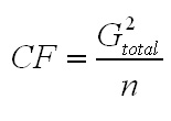 so in this instance: