Kruskal-Wallis one-way analysis of variance [using ranks]

All parametric ANOVA's have to assume that the data is on the Interval or Ratio scales and is normally distributed. In the same way that the Mann-Whitney test provides a non-parametric alternative to the 't'-test, so the Kruskal-Wallis test provides the alternative non-parametric procedure where more than two (k) independent samples are to be compared against one continuous dependent variable and where the data is on the Ordinal scale. As with the Mann-Whitney test, the procedure revolves around the idea of ranking the data and you will see in the SPSS output that each group concludes with a 'Mean Rank'. SPSS deals with this type of data as 'K Independent Samples'.

The KW test does not demand equal sample sizes but it will dictate which post hoc tests can be used.

The data does not need to be in matched groups but if it is, there is a further test, the Friedman test that can be used instead and this method is dicussed later in this Focus page.

The test is frequently used in the analysis of questionnaires.

A market research company have been retained by a pharmaceutical company to carry out a survey of people living and / or working near the production facility. The plant is known to be using toxic raw materials. How do local people feel about this?

Is there any difference in attitudes (perception of danger) between 3 (referenced as: 'k') groups:

• Group k1 those living nearby but not working at the plant (2 mile radius),
• Group k2 those living further afield and not working at the plant (2 - 6 mile radius)
• Group k3 those actually working at the plant

A survey was conducted of the three groups with 10 individuals in each group and their response was given a score and that was recorded on a 1 - 5 scale where 1 indicates that they had no perception of dangers at all through to 5 where they see perceived huge dangers.
The Kruskal-Wallis test statistic is labelled: 'H'.

For degrees of freedom therefore (in this example) we use: (k - 1) = 2

Remember to construct your own H0 and H1 before you begin.

In SPSS open: SPsmAex 04 Factory Chemicals......

In 'Variable view' we have typed in 'case', 'group' and 'score'

and have given 'group' 3 labels: 'live nearby', 'live away' and 'work there'

Go to 'Analyse', 'Nonparametric tests', 'K independent samples'. Tick 'Kruskal-Wallis'.

Transfer 'groups' to Grouping variable and define the range as 1 to 3. Transfer 'score' to 'test variable list', Click 'OK'....

The output should look like this.....

The test statistic (H) is shown to be 9.246.
P = 0.05, critical value (from Chi tables) = 5.991
P = 0.01, critical value = 9.210
P = 0.005, critical value = 10.600

9.246 > 5.991

9.246 > 9.210

9.246 < 10.600

Therefore, as our 'H' value exceeds the first two critical values; our result is significant at the 5% and also just at the 1% level as the output above shows.

The null hypothesis does not hold true and therefore we must accept H1...

"there is a significant difference in attitudes between the three groups"

Important note: we cannot define this discovery in any more detail (i.e. which group with which other group) with this particular test.....

However, just as with the ANOVA test where we used a post hoc test (Tukey's) to distinguish between the three groups; we can do the same after a Kruskal-Wallis test by a number of methods. One to use is the Nemenyi test providing all the sample sizes are equal. There is yet another post hoc test; Dunn's multiple comparison test (not covered here) for use when the sample sizes are not equal.

A large questionnaire / survey was carried out for the IPC, (International Publishing Corporation). It was conducted to see if interest in the Arts and Sciences differed from continent to continent. Such information would help them with their marketing strategy. There is also the opportunity to compare attitudes of both men with women or to compare continent with continent for each gender independently.

The data set is SPex 77 Book publisher

Study the dataset carefully to begin with, note that there are : 2 genders, 4 grouping variables i.e continents, 2 preferences (Arts and Science) and 5 levels of preference response.

Task: Produce 2 boxplots first (the variable will be firstly 'Intoarts' and secondly 'into science', the category axis will be 'Continent of residence' in both cases. Comment on the findings.

Task: Produce your own H0 and H1 before you begin

Carry out a KW test firstly testing the males (gender 1) for their comparative interest in Science and then in the Arts. Repeat the test using (gender 2) females.

In order to separate the gender 1 and 2 data...

In data view, drop down 'data' and click on 'select cases'

Select 'If case is satisfied' and click 'If'.

A new box will open , transfer 'gender' and type in '=1', click continue.

You will see that in your main dataset, the female entries have a diagonal outscore through them all. Thus any analysis willingly take the male cases into account.

So there are 4 comparisons to be carried out: male/intoart, male/intosci, female/intoart and female/intosci. All four tests will be looking for significant differences between the continents.

We can transfer both test variables together but we must deal with each gender separately...

MALE:

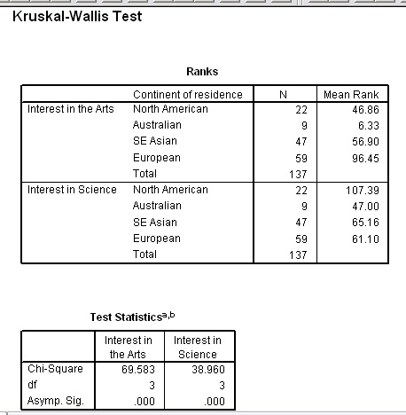
FEMALE:

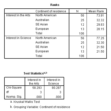
As you can see, the results are highly significant but, multiple comparisons among sub groups (using the same samples all the time) increases the risk of falsely accepting H1 and claiming that there is a significant difference when in fact there is none....a Type 1 error .

We can overcome this danger by utilising an approximation to the Bonferroni adjustment and carrying out a series of post hoc Mann-Whitney unmatched pairs tests. It is then possible to discover whether or not there is a significant difference between any given pair of groups. It is possible to build up a cross tabulated table that indicates all the significance values obtained. We will explore this idea further in the section below when studying the Friedman test.

The Bonferroni adjustment / approximation

There are a number of different methods of making the critical value in a significance test more stringent and this is just one of them. The approximation method used here will reduce the starting critical value (usually 0.05) to a figure related to the number of pair-wise comparisons you have to make.

The adjustment is simply to divide 0.05 by the number of possible pair-wise comparisons that could be made from the dataset.

The formula for calculating other values for the number of comparisons is:

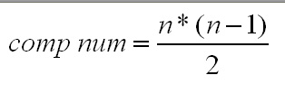
Suppose had run a test with 4 groups (and 3 degrees of freedom), we would divide (P = 0.05) by 6 = 0.0083. There is no particular procedure within SPSS to make this adjustment but the diagram below should show how the idea works.

The 6 pair-wise comparisons would now be undertaken, one at a time using the Mann-Whitney U test but the Bonferroni adjustment would be applied. Thus any output significance greater than 0.0083 would mean accepting the null hypothesis.

The Friedman Test

Much as the relationship between the Mann-Whitney test for unmatched pairs related to the Wilcoxon test for matched pairs; so with non-parametric ANOVA tests. The Kruskal-Wallis test relates to the Friedman test.

These are all tests for Ordinal data.

So essentially the Friedman test is used when you want to use the same sample of subjects or cases and assess them at three or more points in time or under differing conditions.

30 students were assessed each month to see if their fear of statistics was changing over time( as their course progressed) and just before they took the course exam!

Use: Spex 80 Stats exams dataset

Open SPSS, click on Analyze, Non-parametric Tests and K Related samples.

Carry over the 4 variables, tick the Friedman box and click OK

Here is the output:

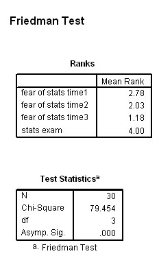
The calculated value for Chi is 79.454   3df: P (0.05) = 7.815 and P (0.01) =11.345
Results are significant if the calculated value is higher than the tabulated value. In this instance, it clearly is.

All of which suggests that there is significant difference in the fear of statistics over time. As the course progressed, it would appear that the level of fear was dropping until the exams loomed when it went back up again!

Another example.....

In a national contest, 10 judges were asked to rank 5 recordings (i.e. cases) of the same song in terms of 'quality of musical interpretation'.

The degrees of freedom are k-1. The null hypothesis would say that there is no significant difference between the rankings achieved by the 5 versions of the song.

Use: SPex 78 music choice

In SPSS, go to 'Analyse', 'Nonparametric tests' and 'K Related samples'

transfer all 5 test variables to the test box, tick 'Friedman' and click 'OK'

Here is the output:

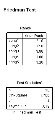
So the calculated value for Chi is 11.76 . 4df: P (0.05) = 9.488 and P (0.01) =13.277

Our result is higher than 9.488 but not as high as 13.277 and as SPSS output shows; it is significant at P=0.19.

It is important to note however that the test has not pin-pointed where (between the various versions) the significant difference lies, only that it exists.
    

Here is a more complex example.....

Many people had lobbied for a long time to get a by pass around the village of Bere Regis. So the local paper decided to investigate local attitudes. 200 villagers(94 men and 106 women) were asked about their attitudes towards a new village bypass.

One question/ statement was worded like this: "The cost and disruption to people and wildlife that the construction will cause is fully justifiable" Do you agree or disagree?

They had to select one of the 5 standard responses on a Likert scale. 1 ='strongly disagree' and 5 = 'agree strongly'

The same people were asked this question before, during, immediately on completion and one year after completion. The initial null hypothesis will say that there has been no significant change in attitude but remember that there are 4 questions so there might be a significant difference between one pair but not another. As with the Kruskal-Wallis test; all we will discover to begin with is whether or not there is a significant difference somewhere in the dataset.

If there is a significant difference shown to exist somewhere in the dataset; we will have to follow the Friedman test with a series of post hoc Wilcoxon tests on each pair / combination. There will have to be a separate null hypothesis for each pair of questions. They will say that there has been no significant change in attitude between Q.... and Q..... H1 will say there has been significant changes in attitude.

Access and study the dataset: SPex 79 New By pass

Women:                                                                Men:

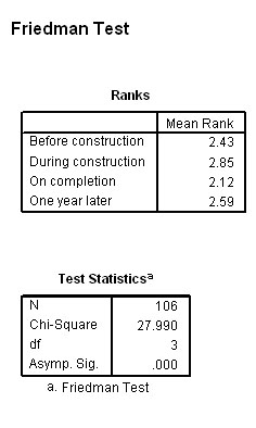
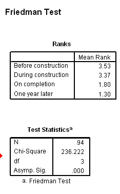
From the mean ranking results, it would appear that the women changed their attitude towards agreement at each progressive stage. The men on the other hand seem to have changed their attitude greatly after construction began. Note the very different Chi values generated.

Applying the Bonferroni adjustment to a series of post hoc Wilcoxon matched pairs tests should allow us to discover where there is a significant difference between the various pair combinations. Again, start with the two rankings that show the largest difference.

Here are the output P values for the 6 male and 6 female comparisons. The non-significant results are shown in blue and the significant results in red.

Remember, for us to accept the alternative hypothesis, the P value has to be less than the Bonferroni adjusted critical value which in this instance is 0.0083

Remember that when SPSS generates a Sig.value of .000, it really means less than .0005. So in this instance that also means less than .0083

Male:

Female:

A different pattern of attitudes has emerged between male and female. To begin with, the men indicated no significant difference between prior and commencement of the works (Q1-Q2) but then significant differences (changes) in attitudes appear throughout. In the case of the women, there was a significant difference between prior and commencement (Q1-Q2) but no significant difference between commencement and completion(Q1- Q3)or between completion and one year on (Q3 - Q4).

Go to 'quick view' contents page

Go back to Focus 13

Go on to Focus 13b