
[Focus 13b] A (very) brief description of some of the other types of Analysis of Variance |
| It is not the intention to give worked examples or to take you through the SPSS methods needed for the procedures outlined below. This is only an introduction. However, they are all classed by SPSS as 'General Linear Models' or GLM's in the drop-down menus under 'Analyse' , 'General Linear Model' and then 'Univariate' (One-Way), 'Multivariate' (more than One-way) or 'Repeated measure' |
All methods of analysis of variance are concerned with examining differences in central tendency where more than two groups are concerned. If there are only two groups for comparison then t-tests, Mann-Whitney test and Wilcoxon tests will suffice... (see Focus 6, 6a and 8).
The data may be in matched groups or not and must be at least on the Ordinal scale. When we want to find out if there is a statistically significant difference among a number of groups, the most common approach is to look at (and compare) the mean values for each group on one or more dependent variables. We started on this path when discussing t-tests. This involved comparing two groups (say male and female) or two sets of data (e.g. before and after) and we compared the mean scores of both.
 The personnel department of Floids Bank are responsible
for the planning of staff training but staff have to be assessed in terms of 'suitability
' in order that the most economic use of educational and training resources are
used.
The personnel department of Floids Bank are responsible
for the planning of staff training but staff have to be assessed in terms of 'suitability
' in order that the most economic use of educational and training resources are
used.
Let us initially try to 'place' a few of the analysis procedures that we might want to use....
| Test Design | Test Variable | Grouping variable(s) |
| One-Way (Factor) ANOVA | Computer software competence | Levels of training given: 6, 12 or 18 hours |
| Job performance / appraisal | Age groups of employees: under 25, 26-40, over 40 | |
| Repeated measure ANOVA | Job performance / appraisal | Age groups of employees: under 25, 26-40, over 40. Tested once and then again after six months and results compared |
| Two-Way (Factor) ANOVA | Computer software competence | 2
levels of training: 9 hours and 18. Gender. (2x2 design) |
| Job performance / appraisal | Age groups of
employees: under 25, 26-40, over 40. Gender. (3x2) design. | |
| Multivariate ANOVA (MANOVA) | Job satisfaction | Gender... and three dependent variables....hours at work,sickness days, time in training, |
| ANCOVA | Job evaluation | As above but adding a 'confounding variable' such as 'number of staff to be managed by the individuals under test' |
| Non-parametric test (Kruskal-Wallis) | Attitudes to customers and the workplace | Gender and Score 5 = 'poor attitude', 4 = 'mediocre attitude', 3 = 'reasonable attitude', 2 = good attitude', 1= excellent attitude'. |
One-Way ANOVA's
One-way analysis of variance (Focus 13) is similar to the t-test but was used when investigating two or more groups. It is called one-way because we have only one independent variable involved. This analysis will tell us if there is a significant difference between the groups but it won't tell us where the significance lies. That is, between group A, B, C, D etc.
Repeated measures ANOVA are similar to simple One-Way ANOVA except that (just as with t-tests) same individuals but measured on two occasions separated by time and / or distance.
| One of the important ideas to grasp with all these more advanced tests is that they allow you to ask more subtle and searching questions. Average values and differences between means do not necessarily exhaust all the hidden information that a dataset holds...... |
We have considered situations where a single value is recorded for each variable within n factors under investigation. Many research programmes and surveys however, need to take readings over a period of time. For example, changes in price, changes in weight, height or speed etc. So the repeated measures may be in time or space or they may be taken on individual sampling units after a series of manipulations. Many laboratory drug testing regimes follow this latter pattern.
So now the ANOVA is going to 'expand' to ascertain whether there is a difference 'within subjects' as well as looking for the variability 'between subjects'. The key point to grasp here is that 'repeated measures' ANOVA operates on the same sample of individuals.... repeatedly.
As a general point, you will note how rapidly a data sets can 'grow' seemingly out of control once we start to introduce more variables into the arena.
Between-Groups or Independent Samples ANOVA presents a situation where we wish to compare the means of two or more independent groups, on the same occasion and with the same continuous variable.
Two-Way (Factor) ANOVA's
Now we move on to a new situation where we have two independent variables, both having an impact on one dependent variable. This is reminiscent of the situation when we looked at multiple regression (Focus 12). These tests also allow for the investigation of any interaction that may exist between the two independent variables. Is one having an effect upon the other?
Once again, there are the Between-Groups two-way ANOVA's and the Repeated measures version.
The one-way ANOVA is very useful but as we have seen, it will only be of use if we need to examine situations involving just one source of variance (such as make of machine). A two-factor design will allow us to examine two sources of variation simultaneously, that is, in the same investigation (e.g. variety of machine and type of customer). Experiments / investigations that examine two or more factors at a time are known as Factorial experiments.
In the business world it is rare that just one independent variable is 'in play' at one time. It is far more likely that many variables are in play and influencing each other in many ways, hence the increasing use of these types of analysis.
On a more practical note, it would seem uneconomic and subject to misinterpretation to investigate one variable in one investigation and then construct a second investigation to investigate the second variable and then onto the third, fourth fifth etc. More importantly, separate investigations cannot show any interactions that may exist between these different variables. It is also quite common for two variables to act synergistically (2 + 2 = 5!) with each other or conversely to act antagonistically (2 + 2 = 3!) .
Remember: for ANOVA requirements any more complex than one-way factor designs, SPSS uses the term; General Linear Models [GLM's].
For
a simple guide to help to select the correct procedure to match your data use
the 'Signpost page' |
Interaction and 'main effect'
In a one-factor ANOVA we generated one F-value....
In a two-factor ANOVA we will generate 3!!
This is because if we have two independent variables (or factors) A and B, then we will generate an F-value for A, an F-value for B and an F-value for the interaction between the two. So if we have two factors to consider then there are three comparisons to investigate....two 'main effects' and any interaction effect. These are the two possible types of effect that can be delineated in a two-factor test.
The
term 'main effect' may be applied to factor A or
B and refers to the effect of that factor on the
values obtained for that
factor...it does not mean 'the largest' or 'the most important'. It would perhaps
be better to think of this as the 'most direct effect'. Thus it would be quite
possible for the two 'main effects' to be non-significant whilst the A / B interaction
could be highly significant.
Study this cross-tabulated 3 x 2 contingency table...
| |
FACTOR A | ||||
| REGIME
3 | REGIME
4 | REGIME
5 | Means | ||
| FACTOR B | REGIME
1 | 35* |
18 |
38 |
30.33 |
| REGIME
2 | 15 |
26 |
22 |
21.00 | |
| Means |
25 |
22 |
30 |
| |
*Note that all these values are likely to be the resultant aggregated mean values of a number of replications of your experiment, market research or survey data.
The large difference between the row means (30.33 and 19.00) might suggest that Factor B was exerting a 'main effect'. Similarly, if a large difference had appeared between the three column means then we would say that Factor A was exerting a 'main effect'.
We now need to understand the idea of 'interaction between factors'. When one level of one factor does not have the same intensity of effect on all levels of the other factor, we say that there is an interaction. We could carry out 6 t-tests but this would be very cumbersome and furthermore, this would actually fail to reveal any effect due to interaction of the two factors.
The interaction between the two factors may be positive, negative or nonexistent.
A 'profile plot' can indicate which is the case....
|
So interaction reflects changes in the ' influence proportionality ' between Factor A and Factor B. Interaction is best detected by producing a 'profile chart'.
If the two profiles are quite definitely not parallel then an interaction is indicated (from table above)...
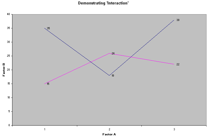
"A clear Interaction" (above)
Multivariate ANalysis Of VAriance (MANOVA)
In this procedure, we can compare the groups in our test on any number of different (but related) dependent variables. Medical research might use this technique to compare different drug treatments on a number of possible outcomes such as blood pressure, heart rate, metabolic rate, brain activity and weight loss etc. MANOVA can be used in a one-way or a two-way situation.
MANOVA can be thought of as an extension of ANOVA.
Do not become confused between the number of cases and the number of variables. All your choices for Analysis depend upon the correct identification of the number of dependent and independent variables to be dealt with...
| How many Independent variables? | How many Dependent variables? | You should use: |
|
|
|
|
| 1 |
1 |
1-way ANOVA |
| 2 |
1 |
2-way ANOVA |
| 1 (or more) | 2(or more) | MANOVA |
Note that in this last case that if the two dependent variables are related to each other (which they usually are) it would not normally be possible to properly determine the effects of the independent variable(s) on any one outcome and hence the need for a MANOVA.
We have to be careful about the null hypotheses also: in an ANOVA' Ho, we are saying "there is no difference between the group means for the variables under consideration".
For MANOVA, we are saying something quite different.....Ho"there is no difference in the sets of means across the groups. Actually, "sets of means" is an over simplification here because we are dealing with multivariate means (Centroids) and the question is whether or not the centroids for each group are significantly apart for significance to be determined. Therefore this is termed the multivariate hypothesis and the rejection or non-rejection will refer to the whole set of variables rather than to any one in particular.
This point can be reasonably illustrated using a Venn diagram but do remember that the circles are intended to represent spheres (i.e. 3D) and not simply circles. The mean might be compared to the centre of a flat disc whereas the centroid may be compared to the central core of the sphere. Perhaps you might consider them as 'flexible gas bubbles' that can change shape, merge and partially cross through each other...
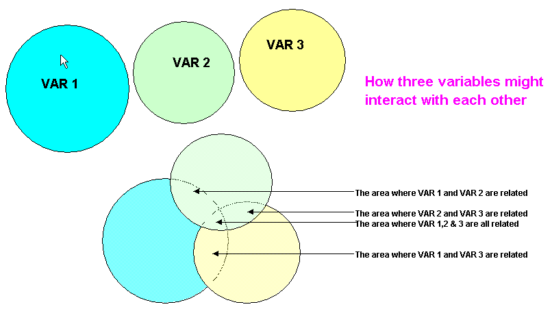
Our previous bivariate analysis methods would have yielded results in the 3 main overlaps (Pearson's Product Moment correlation would yield r-values) but we would not have been able to deal with the central 3-overlap situation. Yet it can be seen that if any one of those circles (variables) changed in size, then the context of the central '3 bubble overlap' would change also. It may be that the 'information' 'buried' in the central '3-overlap' is what we really want to investigate and all the techniques so far discussed will only allow us to look at the three '2-overlap' relationships.
It is not realistic to try to undertake these types of analysis without the use of a powerful computer software package.
ANalysis of COVAriance (ANCOVA)
This type of analysis is designed to reduce the possible effects of a 'confounding variable', that is one that you suspect may have an influence upon the effects exerted by your independent variables on the dependent variable. ANCOVA can be used as part of a one-way, two-way or multivariate design.
Imagine that some biologists were investigating seed production in an Alpine plant species that grows in a variety of different habitats and under differing exposure situations. These factors in themselves can be analysed using ANOVA procedures but supposing that there was a suspicion that 'altitude' may also have an effect upon seed production. The solution would be to widen the investigation and to record the altitude at which all the samples were taken. Thus 'Altitude' become a co-variate. So a co-variate is simply a variable which, although not of direct interest to the investigation, could possibly correlate with the dependent variable that is being investigated.
An ANCOVA may be said to 'purify' the dataset by taking into account the 'new' information provided by the extra set of measurements taken.
![]()
Go back to 'quick view' Contents page
Go on to TOPIC 14