
[Focus
3c; Interactive Page]The Normal Distribution |
To
utilise the excellent interactive capabilities of these graphics, |
The Normal Distribution is the most widely used continuous probability distribution. The curve exemplifies many situations in nature e.g. height of people, the weight of fruit from an orchard of plum trees, germination times from a random number of seeds in a packet, the weights of eggs from a batch of hens etc etc. A ND usually occurs where a large number of independent factors ( e.g.1. heights of the parents, diet, illness etc) are able to affect the outcome.
You will recall that the area under the graph is said to = 1 and in probability terms, 1 = 'certainty' and 0 = 'complete impossibility'. So sections of the area under the curve represent a sliding scale of probability that something may or may not happen.
An important issue is sample size....as the number of samples / pieces of data are added, so the pattern of the Normal Distribution builds up. The normal (or Gaussian) distribution is one of the most commonly observed in nature and in business and is the starting point for modeling many natural and production processes. It usually is found in events that are the aggregation of many smaller, but independent (may be unobservable) random events.
Here is an example, imagine dropping a 1000 balls through a series of pins.....
Drop from here.............................................................V
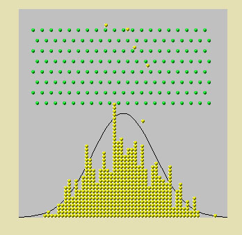
As the balls are dropped from the top they pass through a series of 8 rows of pins until they hit the bottom. Once at the bottom, they stack up to record the number that have hit that point. At first there does not seem to be any pattern but after a few minutes the stacks conform to the superimposed curve. You should appreciate that the probability of any particular ball finishing on the tails is very low and the probability of any ball landing near the mid point is very much higher.
The final position of each ball is determined by many (here only 8) independent, random events of whether to drop to the left or the right of a pin, thus the (approximation) to a normal distribution.
The web link below animates the process that gives rise to the familiar "bell curve" of the normal distribution.
Click the button....
[David
Krider and Mai Zhou are fully acknowledged as the authors of this Applet]
A 'screengrab' from Gary McLelland's website....
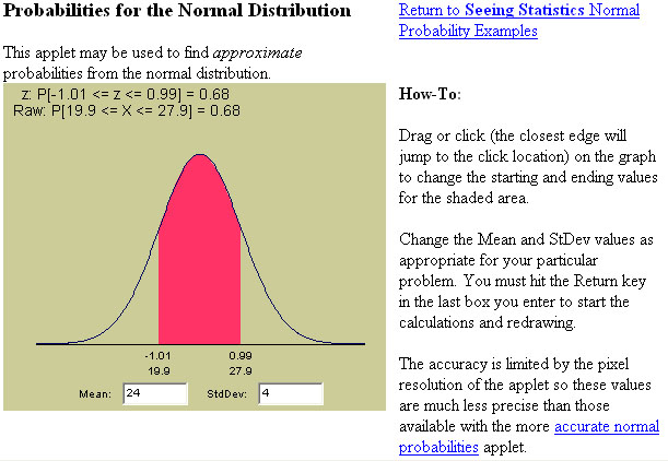
In this instance, the two figures -1.01 & 0.99 represent one standard deviation either side of the mean. The lower figures agree with this in that they show 19.9 and 27.9 (the applet is not yet sufficiently refined to show the precise figures of 20 and 28).
24 ± 4 = range of 1 s.d. either side of the mean i.e. 20 to 28
You will also note that z is given as 0.68 (more accurately; .6826) and is represented as the red area (i.e. 68.26% of the total area) under the graph. That is 34.13% either side of the mean. We can say that in a standard normal distribution, 68.26% of all results will fall within ± 1 s.d of the mean.
Standard deviations away from the mean:
| %
of cases (+ & -) covered | Number
of S.D's away from the mean (left and right) |
|
68.26% |
1.00
+ 1.00 |
| 90% |
1.65
+ 1.65 |
| 95% |
1.96 + 1.96 |
| 95.4% |
2.00
+ 2.00 |
| 99% |
2.58
+ 2.58 |
| 99.74% |
3.00
+ 3.00 |
| 99.9% |
3.32
+ 3.32 |
Try to memorise the figures highlighted in blue as they will be used in future Focus pages.
Follow the link given below, then read the following instructions ....
Use the following link: The Normal Curve in action |
Click-and-drag the left and right end of the red area to change the shaded area under the curve. The formulae in the top left corner calculates the shaded area under the general normal curve for you.
Change the values of the mean and standard deviation, then press 'return' to activate. Familiarise yourself with the relationship between mean and 1 1.5, 2 and 3 s.d.'s above and below the mean.
|
Questions:
Do the probabilities
(areas under the curve) change as the mean and the variance/s.d
vary?
Should they change? Why?
Do the shape, spread, center of the curve change? Why?
[Gary
H. McClelland is fully acknowledged as the author of the above Applet]
Take some time to study the
other 2 Applets available on this website.
![]()
For more about normal distributions go back to Focus 3