
[Focus 4]The Beginnings of Inferential Statistics |
Are two groups different from each other (given Interval or Ratio data)?What is hypothesis testing?P- valuesHo and H1. Type 1 and Type 2 errors
|
Introduction: Our data is always generated from samples taken from a population but what we are really interested in is the population and not specifically the samples .
Inferential
testing offers us an objective route to deciding if any measured differences
or relationships that we have discovered from our samples are truly significant.
Are they real differences or is it more likely that they came about purely
by chance?
Does it mean that the inferences we make are only valid within
the sample or are they a true reflection of what is happening in the wider
population?
In simple terms: does the sample(s) accurately represent the situation within the population and if so, how accurately?
We now need to construct a theory or proposition to decide upon the issue...
| An hypothesis is a proposition (as yet unsubstantiated) which is tentatively held to be true but must be tested to determine if it accords with the facts or not. |
The hypothesis can be worded to determine both the strength and 'direction' of a relationship.
The 'direction of a relationship' needs explaining... If we say that the mean of 'A' is greater than the mean of 'B', we have only indicated one direction for any difference to take. If however, we said the mean of 'A' might 'simply be different from' that of 'B', we are suggesting that this 'possible difference' might be in one of two directions...greater or smaller.
So:
| testing
in one direction only = |
a one-tailed test | e.g.
A is significantly larger than
B |
| testing
in either direction = |
a
two-tailed test | e.g.
A is significantly different
from B |
Hypothesis testing is also concerned with checking on predictions. This may be predictions about differences between samples, predictions about outcomes, predictions about relationships or associations between variables.
With the summary statistics discussed so far, we simply extracted the basic information and moulded it into easily digestible forms.
We are now entering a higher branch of statistics known as inferential statistics.
(1) Our predictions have to be objective. They must not rely upon our personal opinions but on sound mathematical reasoning.
Caution!
When writing
an article, report or piece of prose it is very tempting to use 'statistics' in
a loose and imprecise way in order to strengthen one's argument or point of view.
Avoid doing this! |
(2) Are the differences / similarities / relationships real or could they have arisen by chance?
Hypothesis testing requires us to make a prediction (in a formal way) and then to test statistically how likely it is that our statement is a true reflection of what has been observed or occurred.
The convention is to first write the statement in such a way as to suggest that there is no difference from, no change, no similarity with, no relationship with. You should now know that this is termed the null hypothesis (H0)and is the starting point for all inferential tests. You may like to consider the null hypothesis as the 'default setting' and your task is to test this hypothesis against the alternative hypothesis (H1) to see which holds true.
We always set out by constructing (with very careful wording) the two hypotheses. Data is then collected from the sample(s). The probability that data, or more extreme figures, are a chance result from the sampling is then worked out. With just one sample, the test might be asking "was this sample drawn from the parent population?", with more than one sample, we might ask "are these samples all drawn from the same parent population?"
If this probability turns out to be smaller than the level of significance chosen for the test, then the null hypothesis has to be rejected in favour of the alternative one....
 Britmax Motorcycles plc have two factories, one in Bournemouth
and one in Reading. Both factories have 10 assembly lines. Bournemouth employs
110 assembly workers and Reading employs 154. How do they compare in terms of
productivity?
Britmax Motorcycles plc have two factories, one in Bournemouth
and one in Reading. Both factories have 10 assembly lines. Bournemouth employs
110 assembly workers and Reading employs 154. How do they compare in terms of
productivity?
"There is no significant difference in the mean output per employee with respect to the two factories".
If testing proves unable to confirm the statement made in the null hypothesis then we must reject itit. We would then accept the statement made in the alternative hypothesis.
We also want to calculate how likely it is that our 'snapshot' records give an honest representation of the state of affairs.
"There is a significant difference in the mean output per employee with respect to the two factories"
|
For the null hypothesis (in mathematical terminology & in the case of t-tests later) we can write:

For H0, this indicates that the mean of sample 1 is the
same as the mean of sample 2; i.e. no difference.
The
correctly chosen statistical test will produce a 'test statistic', this will be
compared to a critical value (usually derived from tables). In most cases, if
the test statistic achieved fails to reach the level
of the critical value, then the null hypothesis is accepted. So you may think
of the critical value as a 'pre-set' that allows us to shift from accepting the
null to accepting the alternative.
If the critical value is exceeded, then the alternative hypothesis is accepted in place of the null hypothesis . In othere words, if there is insufficient evidence to accept H0, you must then accept H1, there are no further options.
So we must set our 'pre-set' critical level somehow. Mathematically, this means that we have to decide at what level of confidence we will accept that the null hypothesis is true...Q. On a sliding scale from 'Zero confidence' (a complete impossibility) to '100% confidence' (an absolute certainty), where do you think we should jump from accepting the null hypothesis to accepting the alternative?
When two samples are compared there will be a range (variation within each sample) and a variation between the two samples.
It is always a good idea to try to visualise your data right from the start and this should include producing a chart. Our brain responds much better to pictures than to words. A quick visualisation like the one below can help us to decide what next to do with our data.
Here we can see the use of the 'Box and Whisker' plot again. (see Focus 2b)
The 'box' gives a useful visualisation of the descriptive statistics being worked upon. Remember; the bold line delineates the median and the gold box indicates the position of the 25% (lower) and the 75% (upper) quartiles. Finally, the two 'whiskers' represent the full range of the data set.
Task: Open the data set (SPsmex27 Britmax factories)
Select the 'Graphs' drop down menu and 'Box plots' and 'Simple'
Click on 'Summaries of separate variables' (This is because we want to compare the two variables 'Bournemouth output' with 'Reading output'. Click 'OK'
Caution: If we had pressed 'Summaries of groups of cases' we would have generated a horizontal comparison such as 'Prod 1 / Reading, Prod2 / Reading etc.
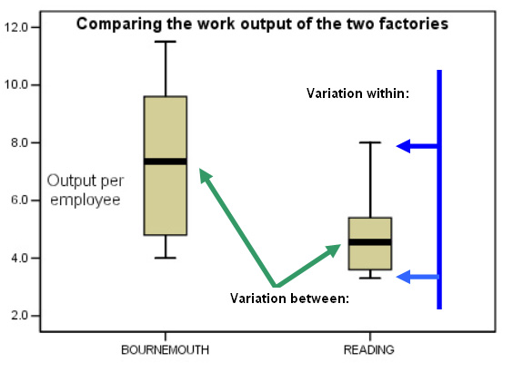
Bournemouth is displaying a higher median value and a larger variation, represented by the height of the gold boxes. We can generally see that the Bournemouth factory is the more productive of the two.
Also note that values between 4.0 and 8.0 units per individual employee actually overlap for the two factories.
We might say that the variation 'between' (green arrows ) is explained by the simple fact that they are two different factories using different management and production techniques. Nevertheless, these two medians are directly comparable because we are measuring the same variable (work output). The variation 'within' (from the lower whisker to the upper one(blue arrows)) is more difficult to pin down; it may be due to the personalities of different workers in each team, incentives, attitudes to work, differences in the quality and efficiency of the tools being used or any number of other external factors.
| Important Rule.... " The larger the ratio indicated by the 'between' and 'within' variations, then the more likely it is that the two means are significantly different". |
Q. Are you able to say that there is or is not a significant difference between the productivity results from the Bournemouth and Reading factories simply by looking at the box plot above?
Statistics can be used to help us describe chance occurrences. The tool we will use is called 'Probability'.......
| 'Probability' has no units and is measured on a scale from 0 (absolute impossibility..... e.g. you will live for ever) to 1 (absolute certainty.....e.g. you will die one day). |
The more likely it is that something will happen; the closer the probability will be to 1. Also, if there are a number of possible outcomes; the probabilities of all of them will add up to 1. Any probability calculation you do will yield an answer between 0.01 and 0.99, if you produce a figure outside of this range, you have done something wrong!
We have already explained that a normal distribution chart can be used to calculate probability because the area under the graph can be assigned a total area of 100 and we know that the 'Y' axis indicates frequency of occurrence. So more individual values occur near the centre of the distribution. This means that any given individual value is more likely to occur here than at one of the tails. Put another way, as we move from the centre towards either tail, the probability of a value appearing gets less and less.
Let us try to see this in a visual way....
 A
hot air balloon is floating over the ocean towards an island in a totally random
fashion. Imagine that the balloonist has 100 footballs on board. When over the
land, he drops one football out of the balloon. The island below is shaped like
a normal distribution curve!!! It comprises exactly 70% agricultural land, 15%
urban development, 10% wasteland and 5% lake.
A
hot air balloon is floating over the ocean towards an island in a totally random
fashion. Imagine that the balloonist has 100 footballs on board. When over the
land, he drops one football out of the balloon. The island below is shaped like
a normal distribution curve!!! It comprises exactly 70% agricultural land, 15%
urban development, 10% wasteland and 5% lake.

Then the probability of that football coming down on agricultural land is 0.7.
To fall on urban or wasteland we add the two fractions together: 0.15 + 0.1 = 0.25.
If we drop all 100 balls, we could set up and test a new null hypothesis.
This would be stated as "There are no external factors influencing the behaviour of the balloon and it is therefore behaving in a totally random fashion".
If indeed 70 balls fell on the agricultural land, 15 balls did land on urban and 10 on wasteland etc, then our null hypothesis would reflect the truth of the situation. The dilemma arises if the ball lands on urban land say 13 times or 17 times and on agricultural land only 65 times. Would the null hypothesis still hold true?
Should we have limits? For example, we may accept that 14 or 16 times still supports the null hypothesis but what about 10 or 20? We are moving gradually further away from the optimum result.
In this type of investigation, we want to know: "what is the probability (P) of the null hypothesis representing the true state of affairs?".
Once a suitable statistical test has been applied to a data set and the calculations made; a test statistic is obtained. Next, we need to know what was the probability of that particular result being obtained by chance. Was it one in ten, one in a hundred or one in a million ? In some cases we might begin at the one chance in ten level, which is expressed as: P(0.1).
Using manual systems (tables) it is conventional to start by setting the 'cut off' point for the null hypothesis to be accepted / rejected at the one in 20 level. In other words...if a result is obtained once in every 20 repetitions, we can put this down to chance but if it happened twice or more times then this would not be chance but a result influenced by a known (or possibly unknown) factor.
This is expressed as: P (0.05) = ####
If we wish to be even more stringent with our conclusions (as is always the case with pharmaceutical trials for instance), then we may wish to use the one in one hundred chance.
This is expressed as: P (0.01) = ####
| 'Chance' |
Expression as a '% chance' |
Expression for
(P) |
| 1
in 100 | 1% |
P (0.01) |
| 1 in 20 | 5% |
P (0.05) |
| 1 in 12 |
8% | P (0.08) |
| 1
in 10 | 10% |
P (0.10) |
| 1
in 5 | 20% |
P (0.20) |
(e.g. 0.05 x 20 = 1)
(SPSS may initially confuse you here because it will always calculate the exact probability (your test statistic) rather than referring to a set critical value but in practical terms, this is more useful as it means that tables are no longer needed.)
Having derived the test statistic value, it is compared with the tabulated value for P at the set level. Then the following statements would apply:
"If the calculated test statistic is less than P(0.05)(tabulated): Accept H0, Not Significant "
"If the calculated test statistic is greater than P(0.05)(tabulated): Accept H1, Significant result"
Viewing this graphically:

Another way to view this is to say "At the 5% level, we will accept the results as significant (i.e. accept the Alternative) only if the result can be shown statistically to have happened by chance in less than five in one hundred times".
 Fabface plc, a cosmetics firm, has just developed a new anti-wrinkle cream.
1000 volunteers have agreed to take part in the consumer trials. 500 are given
the real cream and 500 are given a placebo (dummy) cream to use. The number and
depth of their wrinkles is measured before application. One month later the same
measurements are taken again.
Fabface plc, a cosmetics firm, has just developed a new anti-wrinkle cream.
1000 volunteers have agreed to take part in the consumer trials. 500 are given
the real cream and 500 are given a placebo (dummy) cream to use. The number and
depth of their wrinkles is measured before application. One month later the same
measurements are taken again.
The
null hypothesis will say that: there is no difference in
the number or depth of wrinkles between those who used the real product and those
who used the placebo cream.
The effects (differences in response)
are measured upon all 1000 volunteers.
| Probability: Chosen Critical Level (value found in tables) | Test statistic(S): Value arrived at (by calculation) | What to do with the null hypothesis! | What does this mean in simple language ? |
| P (0.05) value | If
S is more than P (0.05)value | It cannot be accepted and so: accept the alternative hypothesis | It is likely that the differences noted did not occur by chance and are due to the influence of the new cream |
| P (0.05) value | If S is less than P(0.05)value | Accept it as it stands | Any differences recorded could have happened by chance in at least 5 of the 100 volunteers |
You can now see how we can 'set' the level at which we 'switch' from acceptance of one hypothesis to the other. In consumer trials, 5% uncertainty may be accepted, in more crucial trials, such as medical / pharmaceutical trials, only 1% or even 0.1% would be accepted for safety reasons. Imagine a new drug that was likely to cause notable side effects in 5 out of every 100 patients....it could not be tolerated but in 1 in 1000 patients, it may be considered an acceptable risk.
We can now construct a 1- 6 'critical pathway' to guide us through any inferential test procedure:
| 1 |
Decide on the exact wording of the null hypothesis and the alternative hypothesis. Relate this to the original objective of the investigation you are undertaking. |
| 2 | Decide whether a one-tailed or a two-tailed test is appropriate and choose the test accordingly. (Two-tailed are most commonly employed because they look for any difference rather than just greater (or alternatively; lesser) |
| 3 | Calculate the Test Statistic (assume that null is true at this stage) |
| 4 | Compare the resulting Test statistic with the tabular value for P(0.05) and possibly P (0.01) |
| 5 | Accept null or the alternative hypothesis as indicated by the outcome of (4)* |
| 6 | State your conclusions and always relate them to the original hypothesis |
If you adhere to this procedure, you will have a much better chance of producing work that will stand up to scrutiny.
*SPSS gives you the direct level of significance (as a decimal) as stated earlier
The earlier chart is repeated with additional information:
|

The concept of hypothesis testing (and switching at a critical point) has many similarities with a court of Law..
 A jury in a murder trial can return one of two verdicts...Guilty
or Not Guilty. We might say that the "Not Guilty" verdict equates
to our null hypothesis and the alternative would be "Guilty" but in
law, our presumption ( as with our null hypothesis) is always "innocent until
proven guilty" because we can only logically disprove something, not prove
it.
A jury in a murder trial can return one of two verdicts...Guilty
or Not Guilty. We might say that the "Not Guilty" verdict equates
to our null hypothesis and the alternative would be "Guilty" but in
law, our presumption ( as with our null hypothesis) is always "innocent until
proven guilty" because we can only logically disprove something, not prove
it.
Q. Can you absolutely prove that someone is 'not guilty'?
Thus
we always test the null hypothesis and NOT the alternative hypothesis. We test
the hypothesis that the man in the dock is innocent. If we cannot do this, then
he must be found guilty.
However the judge may direct the jury by saying
that he would accept an eleven to one verdict: i.e. at the 91.666% confidence
[P(0.083)] level. Whichever way the verdict goes, the judge would have to say
that the verdict had been arrived at "beyond reasonable doubt". That
means "beyond 91.666%".
If researchers were asked to form a jury, what is the minimum number of jurors they would consider necessary to say "beyond reasonable doubt"?
In the business world it may be acceptable to work with lower levels of certainty but the principle of setting a 'switch point' ( from accepting the null hypothesis to accepting the alternative) is exactly the same.
No verdict can ever be said to be 100% certain and hence the phrase, "beyond reasonable doubt". The same is the case with hypothesis testing...nothing can be proven in the absolute sense but as explained, we can assign a particular level of confidence to our hypothesis statements and this brings us neatly back to our P-values.
The situation can arise where mistakes occur because we have used a 'switch point' that is either to loose or too stringent. We can find ourselves rejecting the null hypothesis when in fact we should have accepted it (Type 1)or visa versa; accepting it when we should have rejected it (Type 2)!
| CRIME / FACT | CORRECT VERDICT HANDED DOWN | ERROR VERDICT HANDED DOWN |
|
"No, the man really didn't do it"
|
NOT GUILTY (NULL) |
GUILTY (TYPE 1 ERROR)
|
| "Yes, the man really did do it" |
GUILTY | NOT GUILTY (TYPE 2 ERROR) |
Type 1 and 2 errors do not mean that you have necessarily made a mistake with your calculations although you may have! A more likely factor here will be your choice of test. Both Type 1 and 2 errors suggest that the wrong confidence level (switch point) has been chosen.
It is worth repeating how important it is to plan your investigations in such a way as to minimise the likelihood of false conclusions being drawn. It is irrelevant how deep the analysis becomes if you start off with flawed data.
| When writing material for public consumption, it is extremely important that you check your facts and figures before allowing them into the public domain. Mistakes and litigation can be extremely damaging and costly. |
We will explore the issues of the pitfalls to be avoided when using 'official' statistics in the next Focus page....
![]()