
[Focus 3]More about Distributions |
Towards the Normal Distribution (N.D)[Visit the N.D Interactive Page]Working with Z-scores(a note about the Standard Normal distribution) |
| Do
be aware that there are a number of other types of distribution besides the normal
distribution. |
By now, it should be clear that most research data that we handle has a number of characteristics which seem to appear time after time. Firstly, if our data is normally distributed and set at the Interval / Ratio level, then this constitutes parametric data....
Caution
! If you are primarily interested
in the analysis of questionnaires, then you are rarely likely to use parametric
/ normally distributed data in your work. |
1) For most of the Interval and Ratio data that you are likely to encounter, the mean is the first focus. Then we examine that data to see if it exhibits (to a greater or lesser extent) a tendency to concentrate on either side of this mean.
2) Remember, if we construct a histogram, the most frequently encountered results often appear about the middle.
3) Less frequently encountered results seem to become less and less common the more we move away from the mean. These less frequently encountered observations / values appear on either side of the mean and are referred to as the 'tails'.
4) If we draw a smooth line through the top and centre of such a histogram, we will produce an approximation to the Normal Distribution curve. There is always only one peak and the shape of the curve is bell-shaped and should be symmetrical. This chart provides a mathematical model that plots the relative frequency of occurrence (on the Y axis) with the single variable under scrutiny on the X axis.
| It may be helpful to think of the normal distribution chart as a special type of histogram where the class intervals are so small that they merge into a continuous pattern. |
There are other situations where the mean value is far to the right or left of the centre. (See 'Skewness') Such cases of 'skew' are said to be positive or negative depending on the direction of the skew. 'Positive skew' would mean that the 'peak' of the distribution curve has shifted to the right.
The term 'kurtosis' refers to the 'peakedness' (or flatness) seen at the top of the curve.
Another special case may be highlighted and that is the 'Standard Normal curve' where the 'bell-curve' is perfectly symmetrical about the mean. Also, in this special case, the mean, median and mode will all be equal.
| Try this
interactive Normal Distribution Curve for yourself.. |
| Virtually all the data sets that are created in the natural world and many in the business world will be normally distributed and whilst it is important to learn about other distributions, for the moment we will concentrate on N.D's. |
It is remarkable just how many phenomena in business, nature and life follow this particular pattern of distribution...
| *The weights of apples on a tree *The weights of strawberries in a punnet *The distances office staff travel to work * The number of invoices handled by an accounts departments *The heights of a randomly selected group of people * The fuel consumption of cars * The ages of all the people at a football match * The blood cholesterol levels in a sample of men of similar age. * The age of people buying new cars etc, etc. |
To repeat:
The main Characteristics of a standard normal distribution are:
|
Learning about z-scores introduces another aspect of normal distribution curves and some of the things they can tell us. We also discussed the '68 - 95 - 99.7' rule; that is the "one, two, three standard deviations" rule in Focus 2. Make sure you are familiar with the theory before progressing here.
Any value on the distribution curve could be given a standardised value in relation to the standard deviation of the whole set so that each observation actually gets its own 'score'...the z-score (note that this is a small z). This score tells us how far away (in standard deviations) that individual score is from the mean, and in which direction.....
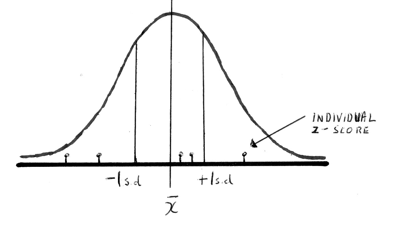
z-scores do have units in the sense that they are "....number of standard deviations", e.g 1.83 s.d.'s. This arrangement allows for a fair comparison of all the individual values under consideration on a fixed and equable scale.
The
simple formula to use is: 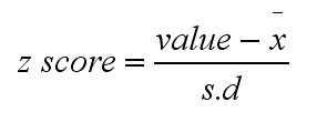
Observations larger than the mean will have a positive z-score and those that are less than the mean will be negative.
Some text books refer to: 'Individual Standard measurements', (ISM). This is exactly the same as a Z-score. (see also Focus 15)
There are 3 examples below to work through....
Ex
1)  Floids bank decides to conduct an aptitude test on 100 of its staff. Here
are a small selection of the marks achieved (out of 100).
Floids bank decides to conduct an aptitude test on 100 of its staff. Here
are a small selection of the marks achieved (out of 100).
| 78 |
| 75 |
| 64 |
| 60 |
| 49 |
How typical are these results of the whole group?
The mean score was calculated to be 68 and the Standard deviation was 6.7. We already know therefore that approximately 68.3% of all the results should be in the range 68±6.7 = 60.3 - 74.7.
So how do these individual scores compare with the mean score achieved by the group? The z-scores for each individual result will tell us. Let us take the score '78'...
78-
68 . .= 10 = 1.49
..6.7 ..........6.7
There are no units attached to the z-score but it is telling us that this individual result is 1.5 standard deviations above the mean. We can also display this result on a normal distribution curve....
 You will see the z-score displayed above the result of 78. You will also be able
to see where this particular score falls with regards to the whole group. The
red area signifies the proportion of all the scores achieved that were less than
78. The area to the right of the dividing line represents the proportion of scores
achieved that were more than 78.
You will see the z-score displayed above the result of 78. You will also be able
to see where this particular score falls with regards to the whole group. The
red area signifies the proportion of all the scores achieved that were less than
78. The area to the right of the dividing line represents the proportion of scores
achieved that were more than 78.
All the scores achieved can be allocated a z-score in exactly the same way.
|
Test Score |
z-score |
| 78 |
1.49 |
| 75 |
1.04 |
| 68 (mean) |
0.00 |
| 64 |
- 0.6 |
| 60 |
- 1.2 |
| 49 |
- 2.84 |
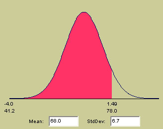
Let us look again at the N.D curve to see where a score of 60 lies on the curve.
 Again, the curve shows us that a score of 60 lies 1.2 s.d's below the mean and
the red area shows the proportion of scores that fall below 60.
Again, the curve shows us that a score of 60 lies 1.2 s.d's below the mean and
the red area shows the proportion of scores that fall below 60.
Ex
2)  A fizzy drinks
manufacturer, Kiddypops Ltd has bought 2 new filling
machines, one for each of their two bottling plants. They need to calibrate these
machines to fill the plastic bottles all to the same volume. The nominal volume
is 250ml but on installing the first machine, it was found to be delivering 257mls.
A fizzy drinks
manufacturer, Kiddypops Ltd has bought 2 new filling
machines, one for each of their two bottling plants. They need to calibrate these
machines to fill the plastic bottles all to the same volume. The nominal volume
is 250ml but on installing the first machine, it was found to be delivering 257mls.
On checking the existing machines the mean 'fill volume' was found to be is 242ml and the standard deviation was 16ml. So how does the new machine compare?
z-score = [257 - 242] ÷16 = 0.938 i.e. almost 1 S.D above the mean.
This should be stated as "the first new machine was delivering 0.94 standard deviations more than the mean for the existing machine in the bottling plant"
Standardising in this way is a form of linear transformation of the data and whilst the true nature of the raw data (mean and S.D) do not change, the technique is very useful for comparing examples from other related datasets or sources.
At the other plant the mean 'fill' from their existing machine was found to be 253ml and the S.D was 9ml....... their new machine only delivered 246ml.
We have the mean volume as 253ml and the S.D of 9ml and a 'fill' value for the second new machine, we could make a legitimate comparison of the two based on their respective z-scores.
So z-score2 = [246 - 253] ÷ 9 = - 0. 777
This should be stated as "this machine was delivering 0.78 standard deviations less than the mean 'fill' volume for the second bottling plant "
We now have the ability to make a direct and fair way of comparing the two machines, albeit on this one parameter alone.
Q. Could we deduce anything useful by simply comparing the mean values of the two machines?
| Remember, a z-scores is a positional index and therefore cannot have any units. It represents a position along the X axis and the greater the ± magnitude of the z score, the further that particular reading is right or left of the mean. |
Just as we were able to say that 68.3% of all scores will fall within ± 1S.D. of the mean, so we can make similar observations about z-scores using the normal curve. 84.1% of all z-scores will be in the range ±2 S.D's. and the remaining 15.9 % will be outside this range. Or we might say that 97.7% of all z-scores will be in the range ±3S.D's and the remaining 0.3% will be outside of this range.
Using the Interactive normal curve (Focus 3c) or book tables, you can check this for yourself by reading the z-score when you move the cursor so that the number of s.d's (red area) is 1 and then 2.
Although we will deal more fully with the issue of Probabilities later. The percentages of the total area (areas under the graph) also indicate the likelihood of a given value(s) actually occurring...
If a normally distributed data set had a mean of 100 and a S.D. of 10...
Calculate the z-score for a value of 110
[110 -100] ÷ 10
=10/10
= +1 & what % of all results would score more than +1....?
...We said that 16% of all results (under a normal distribution curve) would gain a z-score greater than +1 and so the answer....16%!!
Alternatively, study this table which gives the various %'s for each whole number increment of the standard deviation....
S.D's | -4 | -3 | -2 | -1 | 0 | +1 | +2 | +3 | +4 |
area percentages under the graph | 0.13 | 2.15 | 13.59 | 34.13 | 34.13 | 13.59 | 2.15 | 0.13 | |
here
is the 16% ! | |||||||||
| Most text books carry a z-score table (Curwin and Slater p.620 [4th Ed] or p.633 [5th ed] for example) that allows you to look up the specific area under the graph in the Standard Normal Table (usually this will be the area to the right of the z ) and to then deduce what the probability of that score occurring actually is. |
You
will need 'z tables' to do this section, this scan indicates the appearance of
these tables....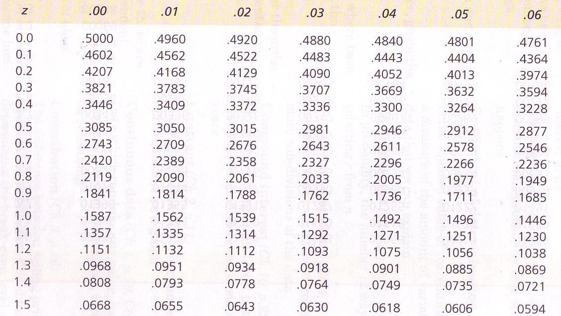
An example:
 A market analyst
is looking at the latest figures from a small film production company.
A market analyst
is looking at the latest figures from a small film production company.
The 2003 accounts reveal that the company achieved a mean turnover (normally distributed) of £11,000 per week and the standard deviation was £2200. All production costs and overheads amount to £8000 per week and this figure didn't alter during the period.
Q. What is the probability of the earnings being more than £12500 in a given week. Use the Interactive Page (Focus 3c) to generate your curve.....
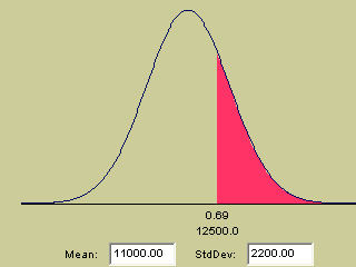 So it is the red shaded area that we are interested in which gives a z-score of
0.69 (although the accurate figure is 0.682).....
So it is the red shaded area that we are interested in which gives a z-score of
0.69 (although the accurate figure is 0.682).....
12500
- 11000 = 1500 = 0.682
........2200
........... 2200
From tables: (Curwin and Slater p.633), read off the vertical z value for the first decimal point and then across for the second. The third decimal point, you will have to estimate as falling between the two adjacent book values. In the scan above, if z were .660; the p-value would be .2546
So
for z = 0.68, the book gives us .2483
for
z = 0.69, the book gives us .2451
So for z = 0.682 we can estimate the p-value
as .2483 -.0006 = .2477
However, for clarity, we will take the p-value as .2483.
Remember our sliding scale? 0 =absolute impossibility and 1 = absolute certainty......
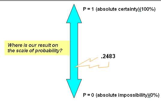
This tells us the probability of the takings being above £12500 in a given week is approximately 1 in 4.
Let us now calculate the Probability of making a profit in any given week.....
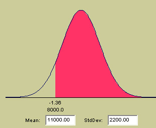 We see that when we set the cursor on £8000 (the weekly costs), the z-score
is -1.36. Check this yourself with a calculator, the full answer should be: -1.3636.
We see that when we set the cursor on £8000 (the weekly costs), the z-score
is -1.36. Check this yourself with a calculator, the full answer should be: -1.3636.
The probability given in the tables for a z-score of -1.36 is .0869 (8.7%). However, this time we are interested in the area to the right of the cursor line. We also know that when calculating Probabilities, that the total area under the graph is taken as 1. So, 1- 0.0869 = 0.9131 or 91.31% . The value of 8.7% represents the probability of not making a profit in any given week.
So
there is a probability of making a profit in any given week of 91.3%.
SPSS can quickly yield all the z-scores for a data set.
Enter all the data (SPSS needs to know the complete range), Click 'Analyse', 'Descriptive Statistics' and 'Descriptives'
Carry your variable over to the variable(s) box
Click 'save standardised values as variables'
Click 'OK'
Your output will appear and the original data set will drop into the systems tray but when you maximise it again you will find that a new column (zvar****) has appeared and these are the complete set of z-values for your data set. It will appear something like this.... (this is not a saved dataset)
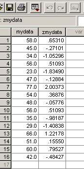
In this data set, the mean was 48.8 and the s.d was 14.07. So the range encompassed by ±1 S.D would be 34.73 and 62.87. The nearest values in the data set are 34 (z =-.98) and half way between 60 (z = .795) & 66 (z = 1.22). The mid point between the two (at 63) is 1.01 !
Q. What do you notice about the z-scores at values of 34.73 and 63? Clue: back to s.d's!
Task: Work out the z-score at 2 s.d's above the mean (i.e. value = 76.95). Clue: look at case 7 in the above dataset
This is the term used in a special case where (mean = zero, s.d. = 1)and is written as: N (0, 1). In the same way that we found z, a standardised value, the same formula allows us to find the standardised variable...notated as capital Z
To repeat the point, classic probability tables in most text books simply list all the probability values(p) for values of z from -3.4 to + 3.4. Use the Interactive Normal curve again.
Going back to the bottling machines example and using the z / probability tables..
| z-score |
Standard Normal Probability | expressed
as a % |
| 0.938 |
.8260 |
82.6 |
| -0.777 |
.7813 |
78.1 |
Take the z-score of 0.938. From z-tables (eg Curwin and Slater 5th Ed , p633) look down the z column to 0.9 and across to .04 (this is the closest we can approximate to 0.938) and you will see a figure of .1736. Add back 4 to approximate to 0.938 gives us a value of .1740. This represents the area to the right hand side of the normal distribution. Take this away from 1 and you will be left with the area to the left i.e.1 - .1740 = .8260 which means 82.6%.
| Remember again, a z-score is a positional index and therefore cannot have any units. It represents a position along the X axis and the greater the ± magnitude of the z score, the further that particular reading is right or left from the mean. |
Task: Now carry out the same procedure using the z-value of -.777.
Back to the bottling plant. Let us suppose that we checked more filling machines
(of the same type) and their 'fill' values were recorded thus:
| Machine |
Level of 'fill' | mean 'fill' for the factory |
S.D |
z-score |
Standard normal probability (p) |
| 'C' |
210ml |
250ml |
45ml |
-0.89 |
.8133 |
| 'D' |
230ml |
" |
" |
-0.44 |
.6700 |
We can even calculate the probability of obtaining a result between 2 z-scores by using table values for p @ z = .89 and z = .44. i.e. take the smaller table value(p) from the larger..0.1433 i.e 14.3%.
More on this subject in Focus 4
| Remember:
a standard normal curve is one that exhibits complete symmetry about the mean and has a mean of zero and a standard deviation of 1. |
Once you have grasped the idea of the frequency histogram, the normal curve and their properties, we can find out more about the frequency of occurrence of cases in different sectors under the curve.
Imagine that we had a data range of 60 - 140, a mean of 100 and a s.d. of 10.
Providing we use a standard normal curve, we can say that: 13.59% + 2.15% + 0.13% = 15.87% of all cases will have a value in excess of 110. Similarly 15.87 % of all cases will have values less than 90. So 31. 74% of all cases fall outside of the range 90 - 110
Q. What % of all cases will yield a value between 90 and 110 (i.e ± 1 s.d)? Clue: Look at the chart below.
This is the point where the ideas of 'frequency of occurrence' and 'probability' come together because we could equally say " the probability of a case occurring with a score in excess of 110 is...... 15.8 times in 100 or 0.158. This last format is the preferred one.
To refresh your memory; the chart below shows the permanent frequency distribution in relation to outward increments in the standard deviation providing that we are using a STANDARD normal curve.
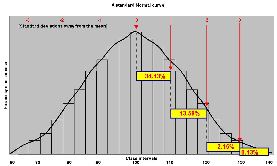
Q. What is the probability of a given value falling between 70 and 90?
To summarise this section....
![]()