
[Focus 7]Working with Index Numbers
|
Index numbers are used widely in the press, in business, financial, sociological and demographic contexts. The principle use of indexing is to make comparisons and in certain circumstances; trends understandable at a glance. Essentially, we must first create a fixed point value (usually adjusted to 100) and then all comparisons both up and down, richer or poorer, are related back to that one fixed point.
Definition: An index number is a statistic that gives the value of a quantity (such as the cost of living) relative to its level at some other fixed time or place. This other time or place value is conventionally set at 100. Using a base figure of 100 is a convenient way of measuring change over time or space. Another commonly quoted definition of an Index is: An Index is a number (with no units) that is used to indicate change in magnitude (e.g. cost or price) as compared with the magnitude at some specified time and usually set at 100. |
The essential point to grasp with respect to index numbers is that we must first devise a 'benchmark'; a standard value for whatever it is we wish to measure and then we move up or down and away from that fixed point.
Index
Numbers are used for a wide range of comparisons in the Finance and Accounting
industries.
Sometimes the comparisons to be made involve large, cumbersome
figures derived from a 'basket' of other figures e.g. GDP. Indexing helps to make
these unmanageable figures manageable.
Here are some of the more familiar ones that are seen in the press and on television:
| Financial Times Share Index | FTSE |
| Dow Jones Index | |
| Retail Price Index | RPI |
| Gross Domestic Product | GDP |
| Unemployment Index | UI |
It is possible to produce an index wherever some quantifiable comparison is required. The mathematics involved are not complicated but care has to be taken to ensure that there is always one clear and well defined fixed point to begin with.
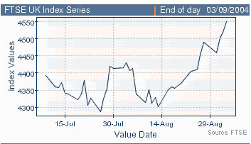
Inflation:If the Government announces that "inflation is running at 4.4%", what this means is that the RPI has risen by 4.4 points from a base of 100 in say June last year to May this year. Next month's announcement will then be based on July last year to June this year and so on. The RPI is widely used in wage settlement negotiations and interest rate decisions. In general terms, the 'health' of a nation's economy is judged by how low an inflation rate it can sustain. In the same way, the Financial Times Share Index (FTSE) monitors the share values of all the companies trading on the stock market and then produces an index of their values measured over time. The current baseline was set to 100 in 1994.
One of the criticisms of the system is that whilst it is easy to follow and sensitive to change; it can become the agent of change in its own right. If investors see prices fall steeply, they will be inclined to sell and this will accelerate the fall. This amounts to a negative feedback system.
|
If
we want to construct an index for the price of one item only, we calculate the
ratio of the new price to the base year price, (called the simple
price relative), and then multiply by 100.
In terms of notation,
s.p.r. =
Pn
x 100
P0
| Year |
1 |
2 |
3 |
| Price
of Item | P0 |
P1 |
P2 |
| £32 |
£48 |
£64 |
| Year |
(Pn
/ P0) | Simple
Price relative (spr) |
| 1 |
32/32 =1.0 |
100 |
| 2 |
48/32 =1.5 |
150 |
| 3 |
64/32 =2.0 |
200 |
 A sports reporter has been checking how the average price of season tickets for
Premier Division football clubs has changed over the past few years....
A sports reporter has been checking how the average price of season tickets for
Premier Division football clubs has changed over the past few years....
First of all, we need to decide which year should be used for the base year and then scale all the figures accordingly. If year 1 was chosen for the base year, we would divide all the prices by 250 and multiply by 100....
| Year |
Price (£) |
Calculation |
s.p.r Index |
| 1 |
250 | (250
/ 250)x 100 = | 100 |
| 2 |
280 | (280
/ 250)x 100 = | 112 |
| 3 |
300 | (300
/ 250)x 100 = | 120 |
| 4 |
320 | (320
/ 250)x 100 = | 128 |
Q. By what % have the tickets increased over the 4 year period?
A second example:
 Here are the number of drink-drive convictions in 'Colliershire' over the
past 6 years.
Here are the number of drink-drive convictions in 'Colliershire' over the
past 6 years.
1999 has been taken as the 'base year' and is therefore assigned
the number '100'.
The year 2000 index will be:(512÷
480) x 100 = 106 .66 (106.7)
| Year |
1998 |
1999 |
2000 |
2001 |
2002 |
2003 |
| Numbers
of cases | 455 |
480 |
512 |
534 |
460 |
470 |
| Index
number | 94.8 |
100 |
106.7 |
111.3 |
95.8 |
97.9 |
At Christmas 2001,
a forceful national media campaign on television and in the press was aimed at
motorists. How effective was it? In
this example, we look at one variable (the number of drink-drive cases), this
generates a simple index . We have compared 'like
with like' and over time. We
need a simple chart to accurately reflect what happened and to present that information
in a fair and measurable way.
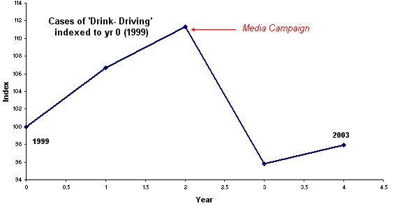
In business and commerce, it is essential that underlying messages and theme are conveyed to staff, clients and the general public in the most effective way. An index chart such as the one illustrated above can achieve this without the audience having to be made aware of the complexities of the original data. The chart above says "this campaign has been a success but note that the problem is increasing again". This is an example where accurate and honest representation of data can be used as an effective management tool to aid reasoned decision-making.
Look at the chart below. You will see that the year 2000 has been taken as the base year. Remember that it is possible to go 'backwards' as well as 'forwards' when working with index numbers. Of course, underlying these seemingly simple index figures would have been the task of collecting a mass of information from petrol and train companies continuously throughout the period and from all parts of the UK.
| Year |
Index of UK petrol
prices |
Index of UK train fares |
| 1999 |
95 |
92 |
| 2000 |
100 |
100 |
| 2001 |
109 |
106 |
| 2002 |
114 |
114 |
| 2003 |
125 |
118 |
| 2004 |
136 |
125 |
| 2005 |
146 |
130 |
It is easy to convert index numbers into charts using Excel.
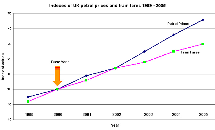
Since 2000, petrol prices have risen by 46% and train fares by 30%. Other % comparisons can be made providing they always refer back to the base year, If two years are to be compared that do not include the base year; then we talk about a "points difference". For example, we might say that "petrol prices went up by 11 points between 2003 and 2004 whilst train fares went up by 7 points in the same period"
So an index is really a ratio or an average of ratios usually involving two 'time points' and the values can be expressed as a %. The resulting value is relative to the benchmark value of 100 but is based on one or more new values collected in the interim. Whatever values made up the original benchmark of 100 remain untouched.
| Caution:
Avoid using the plural term " Indices"...it is more generally associated
with the power of a number. For example with '2 cubed', the '3' would be the index
or "to the power of". In the present topic, we will always refer to:
'Index numbers'. |
|
It is sometimes necessary to compare two index series that have been created using different base years.
 Suppose we wish to track how average house prices have changed compared
to Insurance premium rates. The house prices index has 1999 as a base and the
Insurance Premiums Index has 1997 as a base. So the first task is to decide which
year to take as the joint base year...we decide to use 1999, therefore there is
no need to manipulate this figure but we must adjust the IPI figure to also read
100 instead of 120. This will produce the harmonised index....
Suppose we wish to track how average house prices have changed compared
to Insurance premium rates. The house prices index has 1999 as a base and the
Insurance Premiums Index has 1997 as a base. So the first task is to decide which
year to take as the joint base year...we decide to use 1999, therefore there is
no need to manipulate this figure but we must adjust the IPI figure to also read
100 instead of 120. This will produce the harmonised index....
| Year |
House Price Index |
Insurance Premium Index
(IPI) | Rebased
IPI |
| 1997 |
88 |
100 |
83.3 |
| 1998 |
94 |
116 |
96.7 |
| 1999 |
100 |
120 |
100.0 |
| 2000 |
112 |
123 |
102.5 |
| 2001 |
119 |
127 |
105.8 |
| 2002 |
130 |
140 |
116.7 |
| 2003 |
137 |
144 |
120.0 |
| 2004 |
142 |
149 |
124.2 |
2005 | 146 | 159 | 132.5 |
This is how the figures in column 3 were calculated .......
If 1999 is year one; for rebasing,
the calculation is: 120 x 100 = 1 x 100 = 100
................................................................................................120
and for year two: 123
x 100 = 1.025 x 100 = 102.5
.................................120
and for year three: 127
x 100 = 1.058 x 100 = 105.8 etc etc
....................................120
As usual, a simple Excel chart will help to clarify the information....
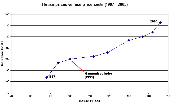
Q. The IPI has increased by 59% between 1997 and 2005 but looking at 2004, have Insurance premiums (Column 4) kept pace with House prices (Column 2)? What is the points difference between the two values shown above?
Aggregated index numbers are produced where a 'basket' of variables are assessed together. The famous 'Retail Price Index' (RPI) is a good example here.
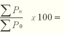
To
include all items, we could sum the prices (year by year) and construct an index
from this sum. If the sum of the prices in the base year is ![]() P0
and the sum of the prices in year n is
P0
and the sum of the prices in year n is![]() Pn, then the
Pn, then the
simple
aggregate price index is given by:
| |
2002 |
2003 |
2004 |
| Items |
P0 |
P1 |
P2 |
| W |
32 | 48 |
64 |
|
X | 60 |
68 | 72 |
| Y |
88 | 92 |
96 |
|
|
180 |
208 |
232 |
| Year |
|
Simple aggregate price
index |
| 2002 |
180/180 =1.00 |
100 |
| 2003 |
208/180 =1.16 |
116 |
| 2004 |
232/180 =1.29 |
129 |
We can go further.....
Note: do not confuse with APR (annualised percentage rate of interest)
Instead of using the absolute prices to calculate an index, we could use their year on year price ratios and treat all price movements as equally important. So the items included could (if necessary) be measured in different units. This method will produce an average price relatives index.
First divide the current year by the base year price for each item. Sum these....
| |
2002 |
2003 |
2004 |
| |
|
Items |
P0 |
P1 |
P2 |
P1/P0 |
P2/P0 |
| X |
32 | 48 |
64 | 1.50 |
2.00 |
| Y |
60 | 68 |
72 | 1.13 |
1.20 |
| Z |
88 | 92 |
96 | 1.05 |
1.09 |
| |
3.68 | 4.29 | |||
....and then divide by the number of items (i.e.3)
| Year |
Calculation |
Average price
relatives index |
| 2002 |
1.00 |
100 |
| 2003 |
3.68 / 3 = 1.23 |
123 |
| 2004 |
4.29 / 3 = 1.43 |
143 |
Such an index is not sensitive to the units used and still ignores the quantities of each item consumed. Up until now, we have allowed all the components that make up an index to have equal status, but this may not always be appropriate.....
 Let
us suppose that on the 1st of January 2000 we bought a specific range of 25 products
from the local supermarket. The checkout bill was £88.91.
One year later we return and buy exactly the same items and the bill is now £94.05.
"Every thing has gone up in price"....but has
it? It is possible that some products have dropped in price whilst others have
increased. The detail in that information will be lost when we produce the 'Index'
but it gives us a 'snapshot' of comparative information about what has happened
in the year.
Let
us suppose that on the 1st of January 2000 we bought a specific range of 25 products
from the local supermarket. The checkout bill was £88.91.
One year later we return and buy exactly the same items and the bill is now £94.05.
"Every thing has gone up in price"....but has
it? It is possible that some products have dropped in price whilst others have
increased. The detail in that information will be lost when we produce the 'Index'
but it gives us a 'snapshot' of comparative information about what has happened
in the year.
In
simple money terms, we can calculate:current year ....x
100 = (94.05 ÷ 88.91) x 100 = 105.8
.............................................................................previous
year
i.e. our 'basket of prices' have increased overall by 5.8%
We have not allowed for the fact that in real life, and over a year, we may purchase far more of one product in the 'basket' than another.
We need an output that gives us not the 'average' or aggregated index of that 'basket' of products but one that is correctly 'weighted' to take account of relative quantities.....
First stage: the individual / simple price Index numbers for each product in the 'basket' of products has to be calculated....
e.g.
Potatoes: Current year .x 100 =
£1.40 ÷ £1.70 x 100 = 82.4
...........................Base
year
| Product |
Base
Year | Current
year | Simple
price Index |
| Potatoes (10kg) | £1.70 |
£1.40 |
82.4 |
| Sugar (2kg) | £2.20 |
£3.30 |
150.0 |
| Meat (250g) | £3.55 |
£ 4.25 |
119.7 |
| Milk (2l) | £1.15 |
£0.99 |
86.0 |
You will note that two products have gone up in unit price and two have come down.
It
is now necessary to assign different 'weightings' to the products in the 'basket'
because the quantities purchased won't be the same and therefore the proportion
of money spent on each item is not equal. The next step is to produce weighted
aggregate index numbers. In business and consumer (retail) research, 'weighting'
is often necessary when considering seasonality and / or fluctuations in demand.
Note:The ratios of the weightings will depend upon the consumption level
discovered for each component. Let us suppose that our research indicated a ratio
here of 2:4:6:5.
That
is; 2 units of potatoes to every 4 units of sugar to every 6 units of meat to
every 5 units of milk.
Second stage: incorporate the weighting......
| Base Index (last year) | Individual Index (current year) | Weighting | Weighted index | |||
| Potatoes |
100 |
82.4 |
x |
2 |
= |
164.8 |
| Sugar |
100 |
150.0 |
x |
4 |
= |
600.0 |
| Meat |
100 |
119.7 |
x |
6 |
= |
718.2 |
| Milk |
100 |
86.0 |
x |
5 |
= |
430.0 |
| Total: |
17 | 1913 | ||||
Divide the total weighted
index value by the total amount of weighting used......1913 ÷ 17 = 112.5
In other words the 'weighted, aggregated cost of food index' has increased
by 12.5 %. The choice of values for the 'weighting' should not be arbitrary and
will depend upon the results obtained by the researcher. In the UK, the Index
of Retail Prices (IRP) monitors over 600 consumable items and the 'weightings',
(product by product), are reviewed annually to embrace changing buying patterns
displayed by the public.
| When complicated figures are simplified in this way there is always a danger of loosing the 'detail' and this has to be balanced against the benefits of being able to deliver clear, concise and accurate data to your audience. |
A second example:
 Here are the mean daily takings for 2003 and 2004 for a
cinema in Winchester presented as Index numbers for each day of the week. Monday's,
Tuesday's, Friday's and Saturdays have all shown increases to varying degrees
whilst the other three days have shown decreases but Friday, Saturday and Sunday
are the most important trading days of the week and are 'weighted' accordingly.
So for example, in 2004, Mondays have shown a 9.5 point increase over Monday's
in 2003.....
Here are the mean daily takings for 2003 and 2004 for a
cinema in Winchester presented as Index numbers for each day of the week. Monday's,
Tuesday's, Friday's and Saturdays have all shown increases to varying degrees
whilst the other three days have shown decreases but Friday, Saturday and Sunday
are the most important trading days of the week and are 'weighted' accordingly.
So for example, in 2004, Mondays have shown a 9.5 point increase over Monday's
in 2003.....
| Base Index (2003) |
Current year (2004) | Weighting | Weighted index | |||
| Monday |
100 | 109.5 |
x | 1 |
= | 109.5 |
| Tuesday |
100 | 111.3 |
x | 2 |
= | 222.6 |
| Wednesday |
100 | 88.7 |
x | 1 |
= | 88.7 |
| Thursday | 100 | 95.5 | x | 1 | = | 95.5 |
| Friday | 100 | 103.7 | x | 4.5 | = | 466.7 |
| Saturday | 100 | 106.6 | x | 6 | = | 639.6 |
| Sunday |
100 | 99.0 |
x | 4 |
= | 396 |
| Total: | 700 | 710 |
19.5 | 2018.6 |
Divide the total weighted index value by the total amount of weighting used......2018.6 ÷ 19.5 = 103.52
In other words the 'weighted, aggregated customer takings index' has increased
by 3.52 points.
If we ignore the 'weighting' component, the index change would be: 710÷700 = 1.0143
= 1.43 points
Task: Comment on the validity and usefulness (or otherwise ) of both results.
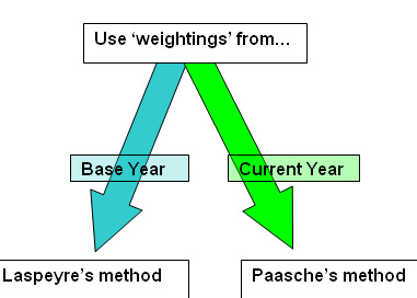
In the above example, we weighted the current year figures and this method creates a Paasche's Index. This index uses the values recorded for the current year. We must multiply each value by the corresponding current year quantity to produce the current year index.
It was stated earlier that it is equally possible to weight the base year figures instead and this creates a Laspeyre's Index. As this index uses the values recorded in the base year, we multiply each new value by the corresponding base year quantity.
A compromise between the two is the Typical Year Index, where the weightings are taken for some time between the base year and the present. This procedure is only used when at least 5 time periods are involved.
 A furniture manufacturer is regularly buying Pine, Beech and Ash timber for stock.
The inward prices (per running metre) in 1998 and 2003 are compared below :
A furniture manufacturer is regularly buying Pine, Beech and Ash timber for stock.
The inward prices (per running metre) in 1998 and 2003 are compared below :
| |
1998 |
Unit quantities purchased
(1998) | 2003 |
Unit quantities purchased
(2003) | Simple
Index |
| Pine |
£1.66 |
5 |
£2.07 |
5 |
1.247 |
| Beech |
£ 2.02 |
4 |
£2.59 |
3 |
1.282 |
| Ash |
£2.66 |
3 |
£3.05 |
4 |
1.147 |
Simple Index e.g. Pine: 2.07 ÷ 1.66 = 1.247 etc. The weightings are ignored.
(1) To obtain the simple aggregate price index:
| (£2.07 + £2.59 + £3.05) | X 100 = 1.216 (21.6%) |
| (£1.66 + £2.02 + £2.66) |
So the prices paid generally by the merchant have increased by 21.6% over the 5-year period but this does not take into account the differential in the amounts of each type of timber purchased.
Caution: be aware of the order in which your calculator deals with algebraic functions. Complete all functions within brackets first and before dealing with numerator / denominator divisions.
The
quantity he buys of each of these timbers varies from year to year but he has
calculated that the purchases in 1998 were in the ratio of 5:4:3 respectively.
So far, there
has been no 'weighting' of the figures.
(2) We will now calculate the weighted price index and use the quantity figures from the base year i.e.Laspeyre's method:
| (£2.07x5 + £2.59x4 + £3.05x3) | X 100 = 1.226 (22.6%) |
| (£1.66x5 + £2.02x4 + £2.66x3) |
The advantage of Laspeyer's method is that the historical figures are readily available but the disadvantage is that the purchasing quantities may have changed and will not reflect the current situation. The timber merchant suggests that he now purchases more Ash than Beech but the same quantity of Pine, hence the ratios are now 5:3:4.
(3) If we use the Paasche method:
| (£2.07x5 + £2.59x3 + £3.05x4) | X 100 = 1.213 (21.3%) |
| (£1.66x5 + £2.02x3 + £2.66x4) |
You may consider that the differences indicated by the 3 methods are marginal. They are not; a 1% difference in raw materials costs could be critical in a business working on low margins or where high volume/low unit price commodities are being manufactured.
Remember:
Using Index Numbers to compare
Salaries with Inflation: |
| 1999 |
2000 |
2001 |
2002 | |
| Annual Salary (£ nett of tax) | 16500 | 17250 | 17750 | 18750 |
| Retail Price Index (RPI) (1993 =100) | 142 |
149 |
155 |
159 |
We need to bring the 2000, 2001 and 2002 salaries back to '1999 pounds'...
Adjusted
2000 salary: 17250 x (142÷149) = 16440.....i.e. <
16500
Adjusted 2001 salary: 17750 x (142÷155)
= 16261.....i.e. 'even less'
Adjusted 2002 salary: 18750 x (142÷159)
= 16745.....i.e. 'slightly >16500!
In terms of 'purchasing power', her salary has not really changed at all.
We know that this index is intended to show the changes in the price of the "average person's shopping basket". Most of the data used comes from the Family Expenditure Survey. It is a good guide to inflation levels in the UK. The weighted average Laspeyre's method is used and the Index is calculated monthly. About 140,000 prices are checked each month and the list is modified to take into account purchasing trends within the economy!
Approximately 16% of a household's weekly expenditure goes on transportation and therefore, the weighting is 0.16. This means that if transport prices rose by 10%, then the RPI would rise by 1.6%. The bigger the proportion of the household income that is spent on an item, the bigger the effect that a price change will have on the RPI.
The weakness with this system is that many groups (such as pensioners) do not conform to the 'average model'. For example, they spend proportionally far more on heating and less on food than the average family. It is for this reason that separate 1-person and 2-person's "Pensioner's Indexes were introduced.
Study the chart below:
| Group |
Commodity |
Weighting |
Annual Increase |
RPI %change |
| Family |
Transport |
.16 | 10% |
1.6 |
| Fuel |
.25 | 12% |
3.0 | |
| Total: |
4.6 | |||
| OAP's |
Transport |
.10 | 10% |
1.0 |
| Fuel |
.45 | 12% |
5.4 | |
| Total: |
6.4 |
The RPI is frequently quoted when revising pensions,
wages and social security benefit payments. The term,"Index-linked"
is often quoted in this context.
(See also example above). Purchasing power is directly linked to the Retail Price Index and can be used to compare the material wealth of the average individual either from a previous time period to the present or in the same time period but between countries.
This useful feature of index numbers (comparing relative values of the same product or variable from all around the world) is illustrated below...
[Care must always be taken that the product(s) to be compared are exactly equivalent otherwise the comparison becomes flawed.]
 The 'Big Mac' Index (first used in 1995)
The
product is virtually identical in all countries in which it is sold, therefore
all factors such as production, distribution, ingredients, exchange rates (between
local currency and the dollar) and
'point of sale' costs are all 'rolled
into' the final retail price.
This type of index is sometimes referred to as a 'Purchasing Power Parity Index'. We could take the 'average' wage of a worker in each country and calculate how many hamburgers one weeks' salary would buy. This would then give us a useful comparison not of wage rates but of the purchasing parity of one weeks' labour in each of those countries. The USA has been taken as the base value...
| U.S.A |
100 |
| Brazil |
116 |
| Canada |
86 |
| France |
166 |
| Germany |
150 |
| Italy |
114 |
| Japan |
200 |
| Mexico |
74 |
| Russia |
70 |
| UK |
121 |
Q. Explain the outcome (in real terms) when a results comes in below 100.
Q. How would you explain the figures for Canada and Japan?
 The Managing Director of Britmax Motorcycles is convinced
that 'pay and productivity' are NOT linked. He has given you the following data
and has asked you to submit a short report after analysing the figures.....
The Managing Director of Britmax Motorcycles is convinced
that 'pay and productivity' are NOT linked. He has given you the following data
and has asked you to submit a short report after analysing the figures.....
Task: Complete the following table and rebase the Productivity Index to 1997. Produce a chart in Excel and answer the MD's question.
|
Year |
Pay | Productivity |
Productivity (rebased) |
| 1995 |
91 |
105 | |
| 1996 |
95 |
105 | |
| 1997 |
100 |
108 | 100 |
| 1998 |
110 |
111 | |
| 1999 |
120 |
109 | |
| 2000 |
125 |
112 | |
| 2001 |
132 |
115 | |
| 2002 |
142 |
118 | |
| 2003 |
150 |
116 | |
| 2004 |
155 |
119 |
[Note that 'Pay' has
1997 as the base year but we have been told that 1990
was used as the base
year for the productivity figures.]
You can access the completed Excel spreadsheet: Britmax Pay Index
The following chart may help you...
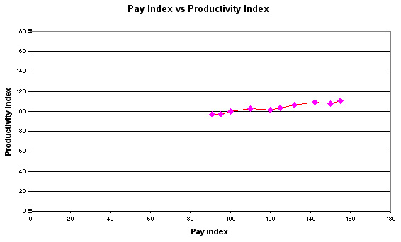
Q. What was the percentage difference between pay and productivity in 2004?
![]()
 A journalist has been looking at her salary slips and assessing her 'spending
power' against government inflation figures. Even though she has had a pay rise
each year; has her salary gone up or down in real terms?
A journalist has been looking at her salary slips and assessing her 'spending
power' against government inflation figures. Even though she has had a pay rise
each year; has her salary gone up or down in real terms?