
[Focus 8]Non-Parametric tests: |
First; more about questionnairesThe Mann-Whitney 'U' test ('U' = unmatched)The Wilcoxon matched-pairs testThe Chi-square test (Focus 8a) |
Introduction
At the end of Focus 6a we looked at the issues of dealing with two data sets where the data was unmatched and we wanted to explore the absolute difference between two means (t-test). We had a situation where the origins and values of the two data sets had grown up independently of each other. If a value in one set alters, it could have no effect upon a value in the second data set.
Also, in an earlier example, Focus 6 (where a fashion store refurbishment programme was being assessed), we could see that the data in the 'after' set was related to the earlier values in the 'at the beginning' set. In that second instance, the paired t-test could be used because the data was genuinely paired, parametric (i.e. normally distributed) and measurable at least on the Interval scale.
We also looked at the idea of ranking data back in Focus 2 where we assessed the overall quality of 'Home Cover' policies offered by 40 Insurance Companies.
More about questionnaires....
Questionnaires are a vital component in studying many areas of human activity today. They can provided clues to the way in which people think, behave and spend their time and money. They can reveal deep seated attitudes to such serious subjects as diverse as abortion, pollution or smoking to more trivial topics such as "what is your favourite breakfast cereal!.
If the questions are designed carefully and the process is given structure, they can provide a standard from which accurate data processing can be derived. Most market research / questionnaire surveys simply do not produce data on the Interval / Ratio scale and so the bulk of the material to be dealt with will be on the Ordinal scale. However, questions concerning numerically-based answers (such as money, age etc) may be analysed using Interval scale methods . You may begin to realise that each question in a questionnaire will have to be analysed individually even if the chain of questions follows a clearly defined thread.
We will explore below how qualitative information (gathered from a large number of individuals) can be processed to show where consensus within the group may or may not be.
Open-ended questions and coding issuesOpen ended questions are often referred to as 'unstuctured' or 'free response'' questions.The researcher cannot predict what the reponse will be. It is usual for such information to be collected verbatim. The style is used for recording likes and dislikes,spontaneous descriptions of products, places or sevices.it is also a useful techniques for collecting information about what changes people would like to see take place. The biggest drawback with this type of question is that it is difficult to analyse in the numerical sense because there are no natural groupings to verbatim speech. Weighting of comments is another problem because some respondents will be more aticulate and verbose than others and yet the opinions of an inarticulate person may be just as valid as those of an articulate person. Many types of question will need to be analysed using some form of coding inorder to 'get the data into the machine'. Manual coding requires a sample of the answers to be examined for their kernal ideas. Commonly occurring themes are then grouuped into what is usually known as a 'code frame'. When the list of 'typical' answers has been identified, each is allocated a code and it is these coded responses that are entered into the dataset. It is also possible to set up pre-coded questions:
The depth and 'quality' contained in the verbatim answer is lost when pre-coding is used but it does simplify the data entry process. SPSS is particularly suited to dealing with questionnaire analysis of most standard types of question.....
|
 Why did you buy that brand of coffee?
Coding for SPSS entry (using variable view)
Before you can enter information from questionnaires etc into SPss, it is necessary to produce a 'codebook'. This is in order that SPSS 'understands' the data entered.
Firstly, each individual variable needs to be named (usally 8 characters are a maximum but SPSS v12 allows more) so make sure that you keep a written notebook with all your abbreviations and acronyms listed so that they do not get muddled.
Next, each response must be assigned a numerical code e.g. Var; Gender: Male = 1, Female = 2.
More complex coding might look like this: Var; Occupation: Student =1, Shop worker =2, Bus driver =3, Nurse = 4, Teacher =5, Pilot = 6 and Window cleaner =7. Note that SPSS places no priorities or seniority to these codes, they are for data entry purposes only.
As mentioned, coding for open-ended responses is a little more complex.
Take the following example: What is your favourite food?
Just
as with the manual example earlier; you will need to browse all the reponses and
look for common themes such as 'Big mac', chocolate, bananas and cream, fish and
chips or steak Diane etc.Using your written codebook, give each grouping of answers
a numerical code. Always add a 'code 9' which is for all answers that do not fit
into your main groupings.
| Answer grouping: | Your coding for SPSS entry |
| Fruit dishes | 1 |
| Meat-based meals | 2 |
| Fast food | 3 |
| Fish-based meals | 4 |
| Confectionary | 5 |
| Others | 9 |
Questionnaire technique is vitally important. Not only must the selection of questions asked be relevant to the interviewee ( there is little point in asking a 15 year old what type of car they drive!) but care must be taken to ensure that the interviewee is relaxed and not irritated or annoyed by the intrusion of the interviewer etc.
| One definition of a Questionnaire: it is a medium of conversation between two people (possibly separated in time and space) and recorded in a repeatable and proscribed fashion. |
Some questions posed can be very subjective...
"Did
you enjoy Jaws 1 more than Jaws 2?" or or " Do people worry more about their Pension plans more than they do about their Mortgage repayments? or "Do you think the BBC licence fee offers good value for money"? etc etc |
 "Is this new cherry soft drink more tasty than the previous one"? or
In fact, all such responses are measurable and can be analysed providing some basic rules are adhered to. The core idea here is that the responses have to be put onto a scale (an Ordinal scale) so that they yield a 'score' and then those 'scores' can be ranked and we utilise the median positions within those ranks for our analysis. Ranks and 'scores' never have any units. Care must be taken not to confuse 'codes' with ranks. Codes have no placings whereas ranks do and all response codes should be given equal weighting. The main use therefore of code-based reponses is to analyse them in terms of frequency of each response.
Remember also that Ordinal data will not yield 'means' but will yield medians. All the calculations are performed on the rank position of each piece of data rather than on the data itself.
A reminder about the ranking of scores:Here are the exam marks for 12 students with the correct ranking shown in column 2
There can never be more ranks than there are data points. Where there are equal scorings, the ranking 'jumps' down to the appropriate level taking into account the number of tied scores. Note also that where three equal scores are involved (as with =6); we could take the mid-value and say that they were in fact =7th. There will be more to learn about median values of rank orders further down this page.
|
Scales and Scaling formats....
There are a number of 'attitude-measuring' techniques used in consumer research and we have mentioned that they should be considered as Ordinal in nature but that some researchers (with little justification) choose to analyse such data as Interval because of the wider and more powerful range of statistical tools available to them. The two most common scales are the Likert scale and the Semantic differential scale....
Likert scale: Mobile phones are the most important
invention of the late 20th century, do you.... Semantic Differential: Mobile
phones are.... It is normal to stay with the idea of 5 levels or divisions |
The somewhat misleading term; scaling format refers to the final way in which a question is 'tailored' to allow the incoming data to be analysed in the most appropriate way. There are more than 10 standard scaling formats but here are 5 of the more common ones ...
Which
hot beverage to you prefer in the morning? Tea [ ] Coffee [
]? (2) Comparative rating. The respondent must rate 'x' against 'y'. (Scaleable) In
terms of your enjoyment how does 'Eastbenders' compare
with 'Concentration Street? (3) Rank Order. The respondent is given (usually n =5) options and has to place them in his/her preferred order.(Scaleable) Rank
the following sports according to your own preferences (1 = least favourite, 5
= most favourite)..... (4)
Checklisting. The respondent is given n options and can select none
to all of them. (Not scaleable but codable) Which
of the following programmes do you watch whenever you can [ tick as many as you
wish]? (5) Determinant
choice. The respondent is given n options and must
choose just one of them. (Not scaleable but codable)
|
Number (3) (Rank ordering) is a particularly useful technique and can be used for making comparisons between two groups. For instance; it is common to use rank ordering to compare attitudes between men and women....
Task: Make sure you are clear about the difference between codes and scaling by devising 4 questions two of which must be Non-scalable and codable and two that are scalable and codable.
Q. What type of input data does not need to be coded
 A new entertainment's complex has just opened in the city centre. The management
want to know if the facilities provided are considered adequate by the 100+ staff.
They decide to assess how satisfied both male and female workers are with the
new facilities. 12 men and 12 women were selected at random to fill in an anonymous
questionnaire.
A new entertainment's complex has just opened in the city centre. The management
want to know if the facilities provided are considered adequate by the 100+ staff.
They decide to assess how satisfied both male and female workers are with the
new facilities. 12 men and 12 women were selected at random to fill in an anonymous
questionnaire.
A question could be structured as follows....
"Our
new recreation complex offers an excellent environment for our staff to work in?"
Place an 'X' in one box only.
| Male/Female |
Phrase |
Tick
one |
| "strongly agree " | ||
|
"agree" | ||
| "neither agree nor disagree" | ||
| "disagree" |
X | |
| "strongly disagree " | ||
This is a 'Likert scale' format.
The next step would be to employ rank ordering and assign a 'score' to each category on a scale of 1 to 5. By adding up the 'scores' given by both men and women; we will gain an overall view of the level of satisfaction. However, the following test method does not do this, instead, we will be comparing the rank order achieved by each possible reply in each group.
Note: it is conventional to use the low scores for the 'least or worst state' and high scores for the 'higher or best state'.
We could also calculate the %'s of men and women that fall into each category. Furthermore, we are potentially able to compare the views from a number of different center's to see if there are any differences in attitudes.
Hence valid comparisons between sets of Ordinal data become possible. We will start with two samples which are independent (and may be of different sizes). This test, the Mann-Whitney 'U' test, is equivalent to the t-tests discussed in Focus 6a but using non-parametric data instead of parametric data. It is still an inferential test and will therefore require a null and alternative hypothesis to be constructed prior to dealing with the mathematics....
The Mann-Whitney 'U' test
Essentially
this is a hypothesis test which sets out to see if
two samples are drawn from populations with the same distribution (that would
be the null hypothesis) or from populations with different distributions (that
would be the alternative hypothesis). If there is a real difference, we
will also be able to superimpose a level of significance to that difference.
There
are a number of conditions to be met before this test can be used.
| 1) The
data has to be at least on the Ordinal scale, i.e. non-parametric data is acceptable 2) Two sample sets are required and the sample sizes need not be the same but ideally, should exceed eight in both cases 3) The two sets must be unmatched / independent of each other. Think of the 'U' as meaning 'unmatched'. One set can have no influence on the data in the other. 4) We always have to use 'scores' (and then rank them) rather than absolute values 5) We will be comparing the median values of the two sets of 'scores' 6) If the sample size is less than 30, tables of critical values have to be used to determine whether to accept the null hypothesis or not. Larger sample sizes are dealt with using a short test based upon the normal distribution. |
You could apply the Mann-Whitney 'U' test to Interval or Ratio data but the 't' tests (Focus 6 and 6a) are more powerful.
Q. Can you explain why?
Remember, if we are dealing with Ordinal data, the measure of central tendency that will be compared can only be the medians .
Remember also: because the data sets are in the form of scores, we are obliged to 'rank them' before doing anything else.
More about the entertainment centre.....
Is there really a difference between male and female attitudes regarding the new facilities?
As usual, we must start with a null hypothesis (H0):
H0 "There is no significant difference between the medians of the samples (male and female) with regards to their satisfaction with the new work facilities.
Task: You phrase the alternative hypothesis.
24 staff members (12 male & 12 female) are asked to fill in the questionnaire(Na = 12 and Nb = 12). Their responses earn scores as follows:
| "strongly agree " | 5 | |
| "agree" | 4 | |
| "neither agree nor disagree" | 3 | |
| "disagree" |
2 | |
|
"strongly disagree " | 1 | |
Here are the derived scores for each respondent:
a) Male |
b) Female |
|
3 |
4 |
| 4 |
3 |
| 3 |
5 |
| 2 |
5 |
| 3 |
3 |
| 2 |
5 |
| 3 |
4 |
| 1 |
5 |
| 4 |
4 |
| 3 |
3 |
| 3 |
4 |
| 4 |
5 |
We could just add up the scores for each set (a = 35, b = 50) but this does not really tell us anything about the significance of these two results. After all, we made up the scoring system to start with. Remember, the Mann-Whitney 'U' test allows us to compare the median values of each group.
Both data sets are now 'blended' together and rearranged in ascending order (column 2 below).
Then an ascending order value is assigned and a median value for each rank (column 4) is calculated.
The rank value will be the mid-point value for a given score respecting the number of values that have gone before. The rank value '8' is derived from the fact that there are 9 records with a score of 3 and they represent the 4th to the 12th scores and the mid point in that range is 8. Naturally, the next group starts at the 13th level.
| |
'Score' | 3) Ascending order position | 4) Rank value |
| M |
1 |
1 |
1 |
| M |
2 |
2 |
2.5 |
| M |
2 |
3 |
2.5 |
| F |
3 |
4 |
8 |
| M |
3 |
5 |
8 |
| F |
3 |
6 |
8 |
| M |
3 |
7 |
8 |
| F |
3 |
8 |
8 |
| M |
3 |
9 |
8 |
| M |
3 |
10 |
8 |
| M |
3 |
11 |
8 |
| M |
3 |
12 |
8 |
| M |
4 |
13 |
16 |
| F |
4 |
14 |
16 |
| M |
4 |
15 |
16 |
| F |
4 |
16 |
16 |
| M |
4 |
17 |
16 |
| F |
4 |
18 |
16 |
| F |
4 |
19 |
16 |
| F |
5 |
20 |
22 |
| F |
5 |
21 |
22 |
| F |
5 |
22 |
22 |
| F |
5 |
23 |
22 |
| F |
5 |
24 |
22 |
|
sigma M = 102 (Ra) sigma F = 198 (Rb) | |||
|
sigma total = 300 | |||
You need to fully understand how to calculate column 4:
Look at the two green rows. The ascending order values were 2 and 3 and there were two scores in this category...
(2 + 3) ÷ 2 = 2.5
and in the next category: 4+5+6+7+8+9+10+11+12 = 72 and divide by the 9 scores in this category
= 8 and so on..
Tip: count inwards using your fingers!!
So now we have a ranked value for each respondent regardless of who it was.
Now go back and sum the rank values (from column 4) for all the men (M) and then separately, all the females (F).
You will find that Sigma M =102 and Sigma F = 198. (Sigma total = Sigma M + Sigma F)
There is a formula which can always be used to cross check that you have done the ranking correctly:
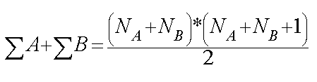
In our case the sum of the ranks is: 300
= (12+12) x (12+12+1) ÷2
= 24 x 25 ÷ 2 = 600 ÷ 2 = 300
The sigma total should be the same at both ends of the calculation.....if they are, we know that our ranking calculation is correct!
The final stage is to calculate the test statistic 'U'. This has to be done for both sets of data because we will have to select the SMALLER of the two values for comparison with the critical value found in the tables.
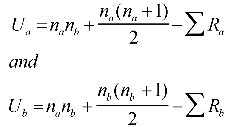
Do not be confused by the use of 'R' in the above formula, it is still the sigma RANK values. The maths becomes quite simple:
'U'a = 144 + ((12X13)÷2) - 102
= (144 + 78) - 102 = 120
& similarly 'U'b = 144 + 78 - 198 = 24
The SMALLER of these two values (24) is our calculated test statistic. It is now compared with the critical value given in the tables.
The Mann-Whitney table is very easy to read; read across and then down for the number of items (n) in both sets. If the samples are of unequal size, the larger of the two must be read across the table and the smaller of the two, downwards. In the above case, na and nb were both 12. Two figures appear: 37 and 27, the first figure is for P(0.05) and the second is the more rigorous P(0.01).
For a significant difference (thereby accepting H1) between the two sets to emerge, the value calculated (in our case: 24) must be SMALLER than the tabular value.
Our value is less than 37, P(0.05) and less than 27, P(0.01) so we must accept H1 and state.....
"There is a significant difference between the medians of the samples (male and female) with regards to their satisfaction with the new work facilities.
This test could now be summarised as follows:
[U = 24, na = 12, nb = 12, P<0.01]
Having established that there is a significant difference, we can go further. The above test was two-tailed and so it only indicated a significant difference; it did not specify in which direction. However, if we look back at the Sigma (M), it was 102 and Sigma (F) was 198. Remember the convention that 'high scores are best state and visa versa'.
So we can now add that the females were significantly more satisfied with the facilities at the new centre than the men were.
Always be aware that the weakness with this type of analysis is the fact that we have 'created' the arbitrary scoring system in the first place and any such scoring system is open to criticism.
Q. Why?
As usual, we will now carry out a similar calculation but using SPSS.
 An independent market research company wishes to gauge the likely levels of user
acceptance of two new types of disc player that have been recently introduced
(Javasound and Purenotes)
to the marketplace by two different companies.
An independent market research company wishes to gauge the likely levels of user
acceptance of two new types of disc player that have been recently introduced
(Javasound and Purenotes)
to the marketplace by two different companies.
Is there any difference in product acceptability between the two products?
Note again that this constitutes a two-tailed approach. We are not asking "Is the Javasound machine more acceptable then the Purenote one" or visa versa. We are simply asking "is there any difference (in acceptability) either way.
Task: Write out an clear and unambiguous null and alternative hypothesis before you begin.
As a pilot study, 30 music journalists were invited to help. They were randomly divided into two groups. One group of 15 'experts' was asked to score the Javasound on a 1- 5 basis and each wrote a single score figure on the card given to them. At the same time, the second group was asked to do the same with the Purenote machine . Product names and labels were removed so that the tests were 'blind' and the experts had no idea which product was which.
Interpretive value of the new pension schemes:
| Descriptive |
'Score' awarded |
| Revolutionary new product | 5 |
| A valuable new addition | 4 |
| A moderately useful product | 3 |
| Of dubious merit | 2 |
| Poor quality, no merit | 1 |
It should be clear that these will be two sets of unmatched data and that the scores achieved by one type of machine has no bearing on the scores achieved by the other.
Here are the results:
Expert: (cases 1-15) | 'Javasound' CD player |
Expert: | 'Purenote' CD player |
| 1 |
4 |
16 |
3 |
| 2 |
3 |
17 |
3 |
| 3 |
4 |
18 |
4 |
| 4 |
2 |
19 |
2 |
| 5 |
3 |
20 |
3 |
| 6 |
5 |
21 |
2 |
| 7 |
4 |
22 |
3 |
| 8 |
3 |
23 |
4 |
| 9 |
3 |
24 |
2 |
| 10 |
4 |
25 |
1 |
| 11 |
5 |
26 |
3 |
| 12 |
3 |
27 |
4 |
| 13 |
2 |
28 |
3 |
| 14 |
4 |
29 |
2 |
| 15 |
3 |
30 |
3 |
| total
score = 52 |
total
score = 42 |
The total scores tell us something; the 'Javasound' machine appears to have done slightly better than the 'Purenote' machine......... but is the difference statistically significant?
Are the total scores really that different ?
Construct your own H0 and H1 and then ...
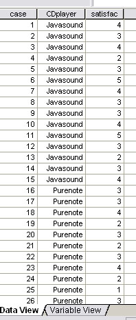
Open SPSS
select 'enter data'
select variable view
Name the variables as: case (for the case number), scheme (for the type of scheme being assessed) and 'satisfaction' for the individual scores achieved.
Similarly, in the Label column, type 'case', 'scheme' and ' satisfac' accordingly
In the values column, give 'Javasound' a label of '1' and 'Purenote' a label of '2'
Switch to the Data View and enter your numerical data.
It should look like this...
 etc
etc
Choose: 'Analyse', 'Nonparametric Tests', '2-Independent samples'
Transfer 'satisfaction' to the test variable box and transfer the Grouping variable (CD player) to the grouping variables box.
Define groups as: Javasound = 1 and Purenote =2
Click: 'continue' & 'OK' to run test
The output should look like this...
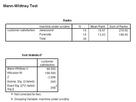
So our calculated 'U' value is 66.50 (SPSS will automatically select and display the smaller of the two values for Ua and Ub) and we should now refer back to the tables (try Wheater and Cook (2000): 'Using Statistics to understand the environment' p.219) for a critical value of Na = 15, Nb =15, P(0.05). The value given in the tables is 64.
Our value is GREATER than the tabulated value and is therefore not significant at the P (0.05) level.
SPSS as above: P> (0.05) i.e. N.S
We must accept the null hypothesis.
The conclusion is:"according to the experts, there is no difference in acceptability between the two machines at the P(0.05) level"
However, note that the output from SPSS is framed in different terms. We are given an exact P value of 0.056 which is greater than the required value of 0.05....i.e. accept H0
Task: The data set is available as SPex 69 CD players. Open it and add the following: 10 more assessors gave their verdicts (5 to each scheme) and these results were added to the previous ones.
'Expert'(cases 31 - 35) | Javasound CD player |
'Expert'(cases 36 - 40) | Purenote |
| 31 |
3 |
36 |
2 |
| 32 |
4 |
37 |
4 |
| 33 |
5 |
38 |
2 |
| 34 |
3 |
39 |
4 |
| 35 |
3 |
40 |
3 |
Task:Re-run the test.....Now what is the conclusion?
Q. Look back at the SPSS output. Why are z- values mentioned in the output?Do not be confused by the inclusion of a 'z' value in the SPSS output. There is a way of calculating 'z' from 'U'. This all relates to a modified version of the 't' tests when large sample sizes are involved and certainly it is the case that as the sample size increases, the probability distribution for both 'U' and 'z' converge. Nevertheless, when presenting your reports (having used a Mann-Whitney test) it is advisable to record 'U', P, Na, Nb, and 'z' |
Carry out this exercise yourself....
 A large book publishing firm
has decided to review its senior management promotions strategy.... Do
the years of experience and hard work really make a difference? Are the number
of years of experience greater in those applicants that get the promotions
than in those that don't?
A large book publishing firm
has decided to review its senior management promotions strategy.... Do
the years of experience and hard work really make a difference? Are the number
of years of experience greater in those applicants that get the promotions
than in those that don't?
30 recent application cases were reviewed, 10 had been successful and 20 unfortunately had not.
Task: Enter the data into SPSS yourself (or use: SPex33 job applicants) and carry out a Mann-Whitney 'U' test to find out.
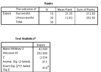
Here is part of the output; interpret it accurately in terms of Ho and H1.
[ The critical value for 'U' (Na = 10, Nb =20 (P 0.05)) is 63]
We have already seen that before trying to make comparisons between two samples we have to address three essential questions in order to decide which test is appropriate.
1) On what scale of measurement is our data ?
2) Are the 2 datasets normally distributed and parametric or non-parametric? (See also Focus 9)
2) Are the 2 datasets matched / paired or unmatched / unpaired / independent?
Task: Learn this table:
| Parametric |
Non-parametric | |
| matched-pairs
(of data) | Paired
't'-test | Wilcoxon
matched pairs test |
| unmatched
/ unpaired / independent | Independent
sample (student's) t-test | Mann-Whitney
'U' test |
We have already looked at 3 of the four combinations and so finally we must look at the fourth test in this particular 'toolkit'; the Wilcoxon matched pairs test.....
The Wilcoxon matched pairs test
| The non-parametric equivalent of the matched pairs t-test |
The Wilcoxon matched pairs test is also frequently used in the analysis of questionnaires and where possible changes in opinion are being investigated. The test is particularly useful for measuring the change in attitudes 'before' and 'after' an event or innovation. In such cases it should be clear that the same people / situations are being compared and that no other factors that might influence the results can be altered. We are not yet ready to look at situations where more than one variable is in play, that comes later!
As with the Mann-Whitney test; both data sets must be ranked and the basis of the test is to discover whether or not the ranking of the actual differences is significant or not.
By comparing the lower of the two rank sum values (the positive or the negative) with a critical value in tables we can say that if our value (T) is greater than the tabular value (P0.05) then we must accept the null hypothesis and say that there is no significant difference.
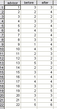
 The management of Tiger FM Radio station have assessed
all 20 of their employees for suitability for promotion. They were each scored
out of a maximum of 20. The top 10 were then sent on a training weekend and were
reassessed on their return. Listed below are their 'before and after scores'.
The management of Tiger FM Radio station have assessed
all 20 of their employees for suitability for promotion. They were each scored
out of a maximum of 20. The top 10 were then sent on a training weekend and were
reassessed on their return. Listed below are their 'before and after scores'.
Has the course been worthwhile or more specifically; has there been a significant change in their suitability for promotion?
Start with the null hypothesis: there is no significant difference between the score achieved before and after the assessment. Write H1 yourself.
Results are only significant if the calculated value of T is less than or equal to the Table value. The diagram below explains this....
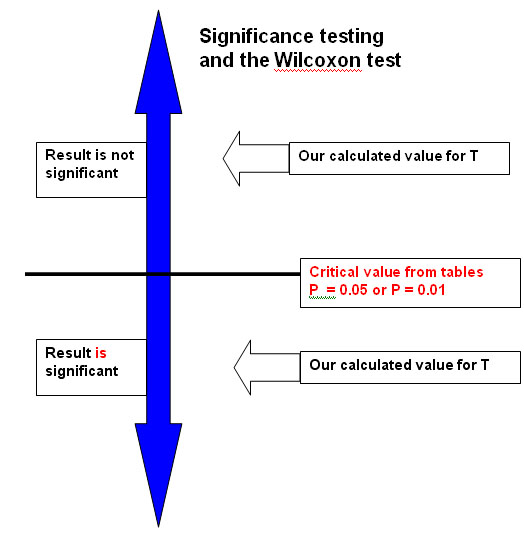
Method:
First calculate the differences in scores (d) for each pair.
"Lowest (d) values first!" Never be tempted to "put the lists in order", remember that the data here is paired and that the pairs must never become uncoupled.
The ranking method: there were four (d)scores of 1, so the mid-point is 2.5 i.e.1+2+3+4 = 10, 10÷4 =2.5
Then recommence at rank 5 because the first 4 places have now been used up. There were two scores of 2 (positions 5 & 6)...mid-point = 5.5 . There was one score of 3 and so recommence at rank 7.
*Any unchanged pairs cannot be included in the ranking......
| Employee: |
'Before' score |
'After' score |
difference (d) |
ranked difference (ignoring the sign) | sign-replaced
ranks (T) |
| David |
11 |
14 |
-3 |
7 |
-7 |
|
Michelle |
13 |
14 |
-1 |
2.5 |
-2.5 |
| Richard |
13 |
13 |
0 |
* |
* |
| Sally |
16 |
18 |
-2 |
5.5 |
-5.5 |
| Tim |
9 |
13 |
-4 |
8 |
-8 |
|
Bridget |
11 |
12 |
-1 |
2.5 |
-2.5 |
| Chris |
18 |
17 |
1 |
2.5 |
2.5 |
| Fiona |
9 |
14 |
-5 |
9 |
-9 |
|
Katherine |
8 |
7 |
1 |
2.5 |
2.5 |
| Emma |
7 |
5 |
2 |
5.5 |
5.5 |
n = 10 [minus any zero values] = 9 and from tables; the critical value (P 0.05) = 5 and (P 0.01) = 2
Sum of the positive signed ranks (T+) = 10.5
Sum of the negative signed ranks (T-) = 34.5.
We select the minimum as our test statistic: 10.5.
The result will be significant if the calculated value is less than the tabular value...
11.5calc > 5tab . We see that the lower T value (10.5) is larger than the critical value (5) and so the probability is greater than 0.05 and we accept the null hypothesis.
We were essentially looking at the median ranked values. The subtle difference this time was the 'matching'. With the 'CD players' example, we had two separate groups of assessors each assessing a specific machine. This time we used one team of assessors but they were judging the same individuals in a 'before and after' situation.
You can access this data set: SPex 70 Tiger Fm staff
A second example:
 The Sagacity software company have developed an updated
version of their online rapid accounting system; 'Sagacity 2'. They say that it
offers 'significant improvements over the older system".
Your company is considering adopting it. However,
there is a marked difference in training and operating costs between 'Sagacity
1' and 'Sagacity 2' . Both pieces of software are to be evaluated with
regards to suitability and you have convened a panel of 16 programmers
who will compare the two designs and give their verdicts on both systems.
The Sagacity software company have developed an updated
version of their online rapid accounting system; 'Sagacity 2'. They say that it
offers 'significant improvements over the older system".
Your company is considering adopting it. However,
there is a marked difference in training and operating costs between 'Sagacity
1' and 'Sagacity 2' . Both pieces of software are to be evaluated with
regards to suitability and you have convened a panel of 16 programmers
who will compare the two designs and give their verdicts on both systems.
Both designs were to be scored on a 1 - 5 basis with 1 being 'completely unacceptable' up to 5 being 'completely acceptable'.
Task: Construct the 2 hypotheses.
It is important to fully understand the ranking method:
There are 7 cases where a score difference (d) of '1' was recorded. Ignore the sign for the time being. The mid-point (median rank value) of this group will have a rank position of '4'. Now we re-commence at rank '8' and look at all those cases where 'd' was '2'....there are 5 and these will run from 8 through 12 and the mid point here will be '10'. Re-commence at 13 and there is only one (d) value of '3'. Re-commence at 14 and again there is only one (d) value of '4'.
Here are the results:
| Programmer |
given score for: 'Sagacity 1' | given score for: 'Sagacity 2' | difference
(d) | ranked difference (ignoring the sign) | Sign-replaced
ranks (T) | |
| |
| |
| |
| |
| 1 |
2 |
4 |
-2 |
10 |
-10 | |
| 2 |
3 |
5 |
-2 |
10 |
-10 | |
| 3 |
1 |
3 |
-2 |
10 |
-10 | |
| 4 |
3 |
2 |
+1 |
4 |
+4 | |
| 5 |
4 |
4 |
0 |
* |
* | |
| 6 |
2 |
5 |
-3 |
13 |
-13 | |
| 7 |
5 |
3 |
+2 |
10 |
+10 | |
| 8 |
1 |
2 |
-1 |
4 |
-4 | |
| 9 |
2 |
3 |
-1 |
4 |
-4 | |
| 10 |
3 |
4 |
-1 |
4 |
-4 | |
| 11 |
2 |
3 |
-1 |
4 |
-4 | |
| 12 |
4 |
4 |
0 |
* |
* | |
| 13 |
5 |
3 |
+2 |
10 |
+10 | |
| 14 |
2 |
1 |
+1 |
4 |
+4 | |
| 15 |
1 |
5 |
-4 |
14 |
-14 | |
| 16 |
4 |
3 |
+1 |
4 |
+4 | |
| T+ = 32 | T- = 73 | |||||
* Caution !! Our usable n figure is 14 (not 16) because 2 cases gave a zero difference.
The final total number of ranks must always take you to the number of cases in the usable data set. That is why in the above situation the top rank is 14 and not 16.
Now re-insert the original ± signs as shown in the last column.
Using this final right-hand (signed ranks) column, we simply add up all the + values and then all the - values and the smaller of the two becomes our test statistic.
T+ = 32, T- = 73. So our test statistic is 32.
The tabular value for P(0.05) (n =14) is 21
We must accept the null hypothesis if our calculated T value is more than the tabulation value.
In this case it clearly is , so we must accept the null hypothesis.
Task: Write a short conclusion statement for the company and include your suggested 'next decision step' ?
Q. If we had used a scale of say 1 to 10 instead of 1 to 5 ; what difference do you think this might have made to the outcome?
You can access this dataset: SPex 71 Sagacity software
Here is 3rd example for you to work through, this time, using SPSS yourself. Remember that the Wilcoxon matched pairs test is very useful in situations where you are dealing with scores 'before' and 'after' an event......
 The government have commissioned an advertising agency to devise a new 'safety
at work' campaign. The media campaign is designed to target factory owners. The
strap line is "be sensible, be secure, be safe"
The government have commissioned an advertising agency to devise a new 'safety
at work' campaign. The media campaign is designed to target factory owners. The
strap line is "be sensible, be secure, be safe"
The
agency have also been asked to measure the effectiveness of the campaign. 220
companies were selected for monitoring purposes.
22 researcher / advisors were allocated to the project..... would they notice any change in attitude from the employers before and after the campaign? Each advisor was instructed to visit 10 companies before the campaign commenced and to interview them all again (the same employers) after the advertising campaign had finished. The advisors had then to give a general overall 'score' indicating the level of safety awareness that they encountered the combined 10 companies that each visited.
A scale of 1 - 6 was adopted with 1 being 'complete indifference' and 6 being 'exceptionally safety conscious'. Here are the 'before' and 'after' final scores submitted by the 22 advisors:
Remember that each 'score' submitted by each advisor is distilled from their findings for all of the managers that each interviewed. So....
Q. Would it have improved our analysis if we had asked for the full 22 x 10 = 220 results?
Q. Discuss how would you re-design this research to give a more robust result?
Open SPSS in the normal way...
Type in your headings in variable view in the normal way
Choose: 'Analyse', 'Nonparametric tests', '2 Related samples'
Transfer the two variables as a pair and tick the 'Wilcoxon' box
Click 'OK'
Task: Interpret the output?
(Remember that in SPSS, 'Z' represents your test statistic)
Task: As Senior administrator, write a short report on the findings for the B.D unit Manager.
Q. In what other ways could you have gauged the success of this campaign?
The data set can be accessed as: SPex 36 factory safety
The next Non-parametric test....Chi square...
Chi Square tests are well known but they come in various guises!!
Firstly, we will consider what to do if our data is not even on the Ordinal scale but has only been collected on the Nominal scale. We must return to the idea of the analysis of frequency data...
![]()
Go on to Focus 8a for the Chi Square page
Go to 'quick view' contents