[Focus 6a]The unpaired or unmatched t-test (Student's -'t')(& a note about Z-tests) |
Caution!
We are still required to use parametric data here |
To qualify as a matched pair (paired data) (Focus 6) we said that there had to be a clear relationship between the two data sets e.g. the same object, the same client, the same exam etc etc. Each pair of values within the dataset had to interrelate in some way and must never be 'uncoupled'....
However, the situation arises when we may wish to compare one bank with another or two airports or two competing supermarkets. They may both be supermarkets but they are in different locations, buy in from different suppliers and have a different customer base.
So
for this test we must assume that the two sets of data are completely
independent of each other;
that one set of values has no direct influence
upon the other. Nevertheless, we must still be working with normally distributed
data.
This
test compares the absolute differences between two sample
means. |
[As always; manual method first]..
 The 'Movietime' Cinema chain wish to compare the
footfall (numbers of people who enter the cinema) in two of their 'metro'
theatres. The method was to record the 3 hour footfall (6pm to 9 pm) figures over
12 days in two theatres of similar size, located 80 miles apart (we have to be
clear that the footfall in one cinema has absolutely no bearing on the footfall
at the other).
The 'Movietime' Cinema chain wish to compare the
footfall (numbers of people who enter the cinema) in two of their 'metro'
theatres. The method was to record the 3 hour footfall (6pm to 9 pm) figures over
12 days in two theatres of similar size, located 80 miles apart (we have to be
clear that the footfall in one cinema has absolutely no bearing on the footfall
at the other).
Also note that we no longer have to have the same number of values for each set because they are not paired. You will note that 'cinema A' failed to collect data on the last day but this will not affect the validity of the test.
The first task in the unmatched 't' test is to calculate the basic descriptive values (sum, mean, variance and s.d) for each set and to square all the recorded values .....
| Survey: 2 hours on.... | Cinema A
footfall values |
xa squared | Cinema B footfall values (xb) | xb squared |
| Mon |
330 |
108900 |
210 |
44100 |
| Tues |
360 |
129600 |
240 |
57600 |
| Wed |
390 |
152100 |
270 |
72900 |
| Thurs |
440 |
193600 |
290 |
84100 |
| Fri |
450 |
202500 |
300 |
90000 |
| Sat |
490 |
240100 |
310 |
96100 |
| Sun |
520 |
270400 |
350 |
122500 |
| Mon |
530 |
280900 |
380 |
144400 |
| Tues |
560 |
313600 |
380 |
144400 |
| Wed |
570 |
324900 |
400 |
160000 |
| Thurs |
580 |
336400 |
420 |
176400 |
| Fri |
430 |
184900 | ||
| Descriptives: |
Mean: 474.5 |
Mean: 331.7 | ||
| Sum: 5220 | Sum: 2,553,000 | Sum: 3980 | Sum: 1,377,400 | |
| S.D: 87.1 |
S.D: 72.2 | |||
| Variance:7587.3 | Variance:5215.2 | |||
na =11, nb =12. d.f = (na -1) + (nb -1) = 21
Q. What is the % difference between the two means and does this give us any indication of the likely outcome?
...to refresh your memory about standard deviation and variance read the box below:
Remember this formula:
Remember
also: The sequence in which you carry out this calculation is crucial. Always work out the term in the brackets first. So, take each value for Xa in turn: 330 - 474.5 = -144.5 and then square it = 20880.25 Repeat the process for the other 10 values in the Xa column. Add the 11 squared values together.... = 75872.75, now divide by (n -1) i.e 10 =7587.275. This is the variance (V). The square root (s.d) of 7587.275 is 87.1 Repeat the who exercise for Xb but remember that (n-1) will now be 12 -1 =11 |
Task: Check out the maths so far with your calculator
We are now ready for the 1- 6 Critical pathway again.
We need a null hypothesis (H0)...
"There is no significant difference in the mean values for the footfall at the two cinemas investigated"
Write out an alternative hypothesis (H1) yourself.
We now need to calculate 't'.
As we are looking for any differences so our test must be two-tailed.
Always begin by making sure that your tabulated data is complete and that you have all the necessary sigma and squared values neatly to hand....
The
full formula (often simplified) is given below. In the subsequent exercise we
will be using SPSS. For now it is simply necessary for you
to follow the steps so that you understand the output when we
get there!
Here we are using 'V' for the Variance.
Although such a formula looks very complex, it is not. Let us work through it step by step....(keep referring back to the table above)
The numerator is 474.5 - 331.7 = 142.8 (leave this figure alone for a moment).
The denominator is the square root of:
(10 x 7587.3) + (11 x 5215.2) ÷ 21
= 6344.77.
The second term simplifies to 23 ÷132 = 0.174.
Multiply
together( 6344.77 * 0.174) = 1104 and then ....
find the square root of this figure: = 33.23
So finally: 't' = 142.8 ÷ 33.23 = 4.297
Our test statistic 't' = 4.297
Check
up in the t tables for 21 degrees of freedom (Why 21?)(Look at the formula above
and remember
that they are independent groups)
at P(0.05) we see the critical value is 2.08.
Our test statistic (t) is greater than 2.08 and so we accept the alternative hypothesis: that there is a significant difference between the mean footfall values for the two cinemas at the P(0.05) level.
Q. At P (0.01) the critical value increases to 2.83. Does this alter the conclusion in any way?
We will now carry out the same test using SPSS.Explanation: There would be little point in starting with an SPSS example if you did not have sufficient understanding to know whether or not the generated output appears correct or not.
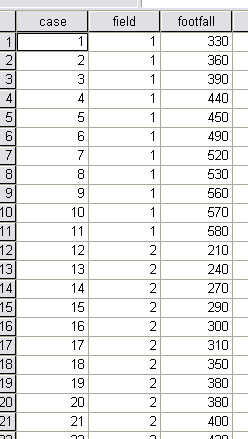
The first task is to enter the data:
Open SPSS
Go to 'variables' view, you need 3 variables
Label cases, field and levels in the usual way
You have 23 cases, now in the Values column(for field) enter '1' for 'Cinema A' and '2' for 'Cinema B'
Switch to data view and enter the data. Your data view should look like this......
We still need to check the data for anomalies so:
Select Analyse, Descriptive Statistic and Explore.
Transfer 'Footfall' to the Dependent box and Field to the Factor box, , ignore 'label cases by'.
Click 'plots' and select 'Histograms'. Click 'OK'
Note: we do not actually need the histograms but a 'box-and-whisker' plot comes with them!
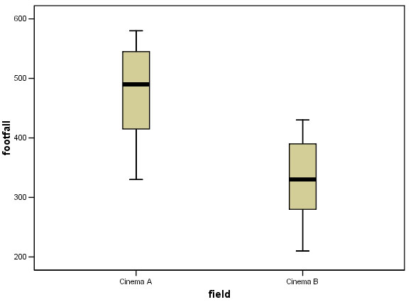
This boxplot shows that there are no extreme values that might affect the outcome
of the unpaired
't'-test so there is no need to leave out any values.
Task: make an assessment of the performance of the two cinemas based on the above chart. Comment on the 'difference between' and the 'differences within'.
We can continue with SPSS...
Choose 'Analyse', 'Compare Means', 'Independent-Samples t-test'.
Transfer
'Footfall' to the Test variable box and 'Field' to the Grouping variable box and
now you will be prompted to
define groups...
Type '1' into the Group 1 box and '2' into the Group 2 box.
Click 'OK' to run the test.
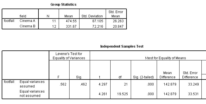
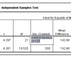
So, t (21 df) = 4.297
Q. Using the highlighted P-value displayed below, showing P< 0.001 but > 0.000; what significance level would you attach to this result?
You can load the data from: SMex 07 footfall
| A
note of explanation is needed here concerning Levene's test
for equality of Variances. Providing Levene's test gives a value for P>0.05 (and in this instance it does), the equality test result is not significant and we therefore assume equal variances apply to our dataset. Thus we use the top row. Conversely, if P<0.05, then equal variances cannot be assumed and we would have to use the lower line. |
So our calculated 't'-value is still 4.297
The table value P(0.05)(21df) is 2.080
The table value P(0.01)(21df) is 2.831
Remember: The result is significant only if tcalc is higher than ttables
Q. So what conclusions can be drawn? Does this agree with the information in the chart above?
 A financial
analyst for the Sunday Bugle is comparing the prices
of a selection of 'Home Plus' policies offered by two well-known on-line Insurance
Brokers. He is attempting to find out if the two companies offer similar deals
or whether one offers better value than the other. The range of quotes must all
fall in the range £40 - £120 premium per month. All parameters such
as level of building cover, personal effects and contents cover remain the same
throughout.
A financial
analyst for the Sunday Bugle is comparing the prices
of a selection of 'Home Plus' policies offered by two well-known on-line Insurance
Brokers. He is attempting to find out if the two companies offer similar deals
or whether one offers better value than the other. The range of quotes must all
fall in the range £40 - £120 premium per month. All parameters such
as level of building cover, personal effects and contents cover remain the same
throughout.
15 examples are collected from each Broker's website.
Task: Remember to write the null hypothesis and the alternative....
Enter the data for yourself in SPSS. Note once again that we have to assign a number to both independent variables (the brokers) so label Broker A as '1' and Broker B as '2'
If you have difficulties; the dataset is: SPsmex 08 Brokers
Again, check the data first for anomalies so:
Select 'Analyse', 'Descriptive Statistics' and 'Explore'.
Transfer 'Monthly Premiums' to the Dependent box and 'Broker' to the Factor box, ignore 'label cases by'
Click 'plots' and select only 'Histograms', Click 'OK'
Note again : we do not actually need the histograms but a 'box-and-whisker' plot comes with them and is very useful !
Generate the following Box Plot.....
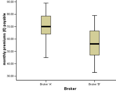
You
should by now be able to interpret the box plot quite accurately and this will
help when evaluating the results of the SPSS output. Now run the test as before
and complete the following
charts..
| Broker 'A' | Broker 'B' | Combined | |
| Mean (£ monthly) of a 'Home Plus' Policy | |||
| S.D. |
| critical value for: 't'tables (P 0.05)(28df) | 2.048 |
| 't'calc | |
| df | |
| P |
Task: Write a short article for the paper and suggest how this investigation could be made more meaningful. Was there a significant difference or not and if so, at what level?
[You will need to know that the critical values from tables: P(0.05) = 2.048 & P(0.01) =2.763]
 In Focus 4, we compared the work output from two groups
of assembly workers in two individual motorbike factories.
In Focus 4, we compared the work output from two groups
of assembly workers in two individual motorbike factories.
The descriptive statistics again ....
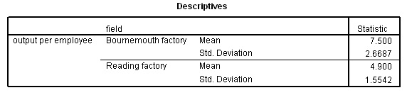
The question under consideration is:"is there a significant difference between the two means shown above?
Task: Use dataset: SPsmex 29 Britmax~2 to produce the following Box Plot (as described above using 'Explore'). Note also that there are 3 variables and that the second variable (field) has two values: '1=Bournemouth' and '2 = Reading'.
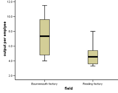
Having noted that there are no outliers to be dealt with....
Choose 'Analyse', 'Compare Means', 'Independent-Samples t-test'.
You should be able to follow earlier examples to complete the test. Start by writing out your null and alternative hypotheses.
Here is part of the final output....
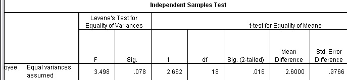
The t value is shown to be 2.662 and the p-value is < 0.05 but > 0.01 (actual: 0.016).
Q. Is 't' significant at the 5% or 1% levels or at some other (following normal conventions) level?
There
is one situation where the use of the unmatched t-test can be supplanted.
If either sample set exceeds 30, then a Z-test can
be used. The Z-test makes use of z-values and their relationships within a Standard
Normal Distribution.
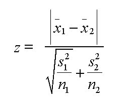
Study the formula below, see how it is constructed
to interpret the absolute difference between two means and to ratio that difference
against the combined standard deviations.
The calculated test statistic (z) is compared with critical values from 'values of z' tables (Wheater and Cook(2000) p217. As
before, the result is significant if your calculated value of z exceeds the tabulated
value.
|
The
formula simply requires the 2 means from the two data sets and the variances (here
indicated
by S˜) (remember: variance = standard deviation squared). Both
sample sizes: (n) are also required
but, as with the unmatched t-test, they
do not need to be equal....
Returning to
'Movietime' cinemas ....although the sample sizes
are not
technically large enough to warrant the use of the Z-test, we can
demonstrate that the outcome should mirror the outcome from the t-test. (Where
we found tcalc = 4.297).......
using the Z-test instead, the following outcome is obtained:
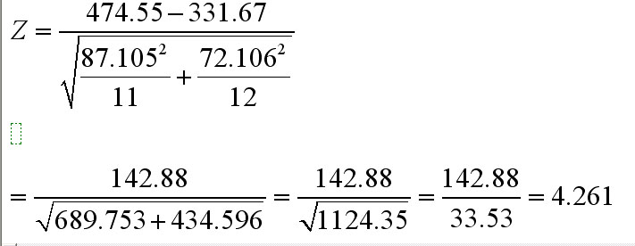
The test statistic (z) = 4.261. This value exceeds the P(z)(0.001)tab value of 3.291 and is therefore significant at the 99.9% level....just as it was using the unmatched t-test.
TASK: Carry out a Z-test on the two Insurance Brokers example. How do 't' and 'z' compare this time?
![]()