
[Focus 17] Binary Logistic Regression |
Logistic regression is used to predict membership of categories a nominal (i.e. Categorical) and usually dichotomous (e.g yes /no) dependent variable from a set of any initial number of (co-variate) predictors. The hypothetical chart below summaries this point....

Normally,
with a categorical dependent variable, discriminant function analysis would be
employed if all of the predictors are continuous. However, Logistic regression
is preferred to discriminant analysis if the predictors
are a mix of continuous and categorical variables.
Logistic regression makes no assumptions about the distributions of the predictor
variables. This procedure has become especially popular with medical research
in which the dependent variable is..... whether or not a patient has a disease....
yes /no?
Logistic Regression is similar to Discriminant Function analysis
in that it represents yet another approach to category prediction
but entails fewer assumptions than discriminant analysis does. It is therefore
often preferred as a method where Discriminant analysis is deemed unsuitable.
Ultimately, logistic regression can be used to predict category membership given
the predictor data for each case. We can also assess how reliable that process
is as a % accuracy just as we did with Discriminant analysis.
We have to start with the concept of finding out the level of success achievable in predicting group membership before undertaking any analysis. In fact, a prediction of category membership can be made without doing any regression analysis at all....
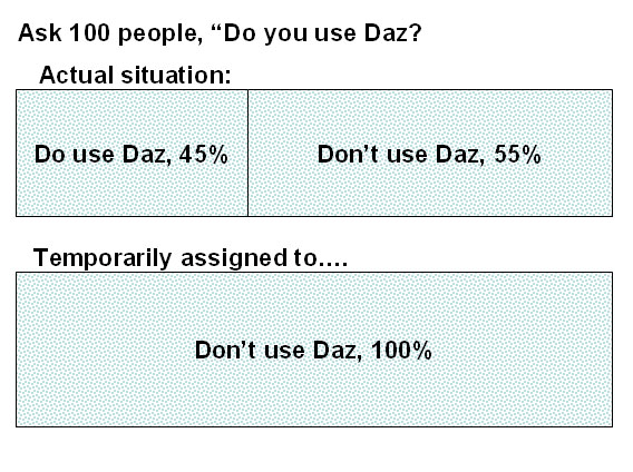
 100 people were interviewed concerning which washing powder they used. One question
simply asked "Do you use Daz? Y/N. The respondents were to be categorised
into two groups depending solely upon whether they use Daz or not. So the 'Y/N
grouping' becomes the dependent variable.
100 people were interviewed concerning which washing powder they used. One question
simply asked "Do you use Daz? Y/N. The respondents were to be categorised
into two groups depending solely upon whether they use Daz or not. So the 'Y/N
grouping' becomes the dependent variable.
45 do use Daz and 55 do not.
However, we may wish to discover what is influencing that decision and hence dictating the grouping that an individual finally ends up in. If we can do that with a high degree of accuracy, we could then go on to predict which group a new untested individual should fall into once we know the values for the independent parameters chosen as they mathematically relate to that new individual.
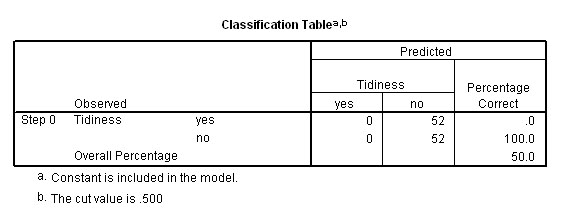
The probability of selecting any one person (out of 100) at random that does use Daz is .45. The best prediction of category membership of a randomly selected person would be to assign them all temporarily to the "Don't use Daz" category. If we did this, we would be right 100% of the time in those selections where they actually don't use Daz but wrong in only 45% of those instances where they do use Daz.
Our overall prediction success rate is therefore only 55% (see drawing below). However, this is our best success level of prediction, so initially we will assign all members to this group.
There may well be factors that influence the decision to use this product or not e.g. price, preferred wash temperature,etc and these would be the independent (or predictor) variables and they are continuous variables.
Logistic regression attempts to improve on this performance by gauging the levels of association between this dependent and the selected influencing independent variable(s). Part of the SPSS computer routine will be to deselect and reselect those predictor variables that are actually influencing the dependent variable sufficiently to stay in the calculation.
In SPSS, the output would appear thus...
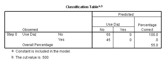
So, overall, we would be right 100% of the time with regards to people in the 'Don't use' category but wrong in 45% of those actually in the 'Do use' category. So the best we can hope for will be to be correct 55% of the time. Logistic regression sets out to improve on this 'no test' approach.
The actual mathematics are quite complex so we shall move on to using SPSS to see how the procedure works in practice.
 100 male students filled in a questionnaire about their
smoking and drinking habits. They were
asked to score themselves (honestly !) as follows: 10 cigarettes per day = 1 smoking
unit and 1 pint of beer = 2 alcohol units. They were also asked if they had suffered
recently from a chesty cough: Yes / No? The preliminary descriptive analysis revealed
that 48 students (48%) had a cough and 73% of this group smoked. Within the group
with no cough, only 9.6% smoked. There was no apparent pattern with regards to
alcohol consumption at this stage.
100 male students filled in a questionnaire about their
smoking and drinking habits. They were
asked to score themselves (honestly !) as follows: 10 cigarettes per day = 1 smoking
unit and 1 pint of beer = 2 alcohol units. They were also asked if they had suffered
recently from a chesty cough: Yes / No? The preliminary descriptive analysis revealed
that 48 students (48%) had a cough and 73% of this group smoked. Within the group
with no cough, only 9.6% smoked. There was no apparent pattern with regards to
alcohol consumption at this stage.
With the Y/N answer becoming the dependent variable (i.e on the nominal scale) it should be obvious that simple regression cannot be used here but binary logistic regression can cope with both qualitative as well as quantitative variables.
Use SPex 81 Student habits and remember that we are not trying to prove anything here but we are simply trying out different ways of exploring the dataset and in particular, we will attempt to predict category membership.
So to begin with, let us check relationships with a Pearson's correlation test. See also Focus 10a
Open
the dataset, drop down 'Analyse', 'Correlate', 'Bivariate' and tick 'Pearson'
and 'two tailed'.
Tick 'Flag significant correlations'
Transfer all three
variables to the variables box.
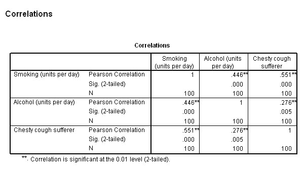
Category membership seems to be quite strongly correlated with smoking (rp = .551) but much less strongly correlated with alcohol consumption (rp = .276). The level of smoking and drinking are also significantly correlated (rp = .446).
| Note that using such correlations when only two states (instead of 3, 4 etc) of the dependent variable are present (i.e.Chesty cough Y /N) can give misleading results. |
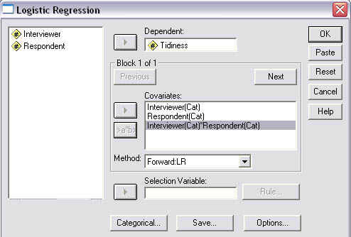
The SPSS procedure:
Drop
down 'Analyse', 'Regression', 'Binary Logistic'
Place 'chestcof' in the
Dependent box and 'smoking' and 'alcohol' in the covariates box.
Rehighlight
both of these two latter variables together and the interaction [>a*>b]
button will activate.
Click this button to transfer the interaction term to
the covariates box. This is done in order to explore whether the effects of one
of the independent variables is compounded by the effect of the other.
Change
the default Method box from 'Enter' to 'Forward FR' This is because the latter
shows more clearly which variables are entered and which are finally excluded
from the analysis.
Click 'Options', 'Hosmer-Lemeshow goodness of fit',
under residuals, tick 'logit' and 'Iteration history'. Click 'continue'
Click
'save' to open yet another dialogue box, under predicted values, tick 'group membership'
and 'probabilities',
Click 'continue'
Finally, click 'OK'.
The
output is extensive (19 tables!) but let us see if the exercise has been worth
doing in the first place. Have we actually raised the level of predictability
accuracy by carrying out this procedure?
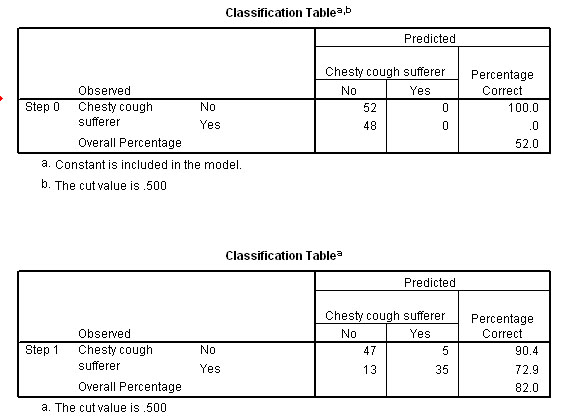
Answer: Compare outputs
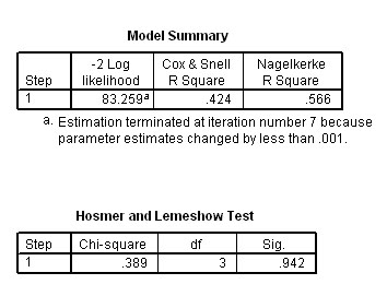
5 and 13......Yes! From 52% accuracy at then
regression applied' (Step 0) to 82% accuracy (Step 1) when the full regression
model was applied to the data. This 30% jump represents a major improvement in
our prediction capability.....
Next look at output 7, Iteration History, this summarises a complex computer process that reappraises the predictions of group membership a successive number of times until the estimates converge to a point where they become almost constant and stabilise, in this instance the Coefficient constant stabilised at -1.313.
If the iteration history does not stabilise then the analysis will not work anyway and other lines of thought should be investigated. A good analogy here would be to imagine that you are focussing the lens of your camera by continually adjusting it and when satisfied that the image is in focus, you stop adjusting things and take the picture. In this case, the computer stopped adjusting the model after 7 iterations.
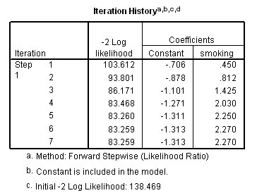
Notice that the only variable selected was 'smoking' and that 'alcohol' was never added. The interaction 'smoking*alcohol' was also never added.
Table 9 gives a number of statistics that mirror the co-efficient of determination in simple regression. You will notice in particular the Nagelkerke R square figure of .566. This value is on a scale of 0 to 1 and is an indication that the regression model that has been constructed has added a major contribution to the prediction of any case having a chesty cough or not.
Table 10, the Hosmer and Lemeshow test has yielded a low value for Chi and a high p-value. This also confirms that the model created fits the data very well. For a good model fit, the requirement is for a low, insignificant value for chi-square.....
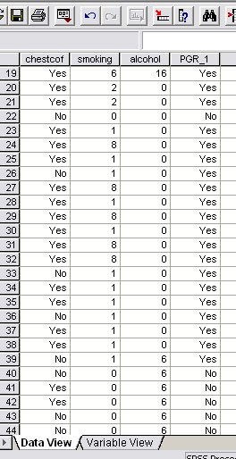
Next, go back to the original dataset and you will see that a new column of saved 'predicted group membership' (PGR_1) has been added. On the screengrab below, only cases 26, 33, 36, 39, 41, and 42 are wrongly predicted. As stated however, with no analysis, the best we could have achieved would have been a 52% accuracy and now it is 82%.
We are also able to construct an equation and output 17 lists the coefficients for what is called the logit equation.....
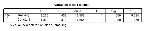
Interpreting this table is similar to the interpretation used in simple regression:
Estimated logit value ('score') = (2.27*smoking) -1.313
Now go back to the data set. Remember that we ticked the Logit box and the 'save options. This meant that the 'scores' for each case have been saved as LRE_2.
Go to the drop down Data menu and select 'sort cases' and sort by LRE_2
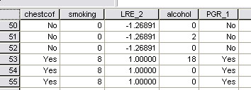
Task 1: Study the extract from the completed spreadsheet. The columns have been rearranged to help. What do you notice about the Logit Regression scores in relation to the values for the two predictor variables? Write a paragraph of explanation for a fellow student.
Task 2: Study the whole data spreadsheet carefully and deduce the relationship between the figures and the values in the Smoking and Alcohol columns. Is it only the Smoking values affecting the logit value? Do the alcohol values have any effect?
Our main conclusion would be that smoking alone increases the liklihood of having a chesty cough. Of the 48 cases who did have a cough,the analysis correctly identified 35 of them. There were 13 cases who had the cough but did not smoke. Of the 52 who did not have the cough, the analysis correctly identified 47 of them. The correlation between cough and smoking (.551)was shown to be significant (p< 0.01).
Furthermore, in 82% of the cases examined, we could have predicted the presence or absence of a chesty cough simply based upon their cigarette consumption.
Interpretation of the Regression constant and the Regression coefficient(s)
 The probability (p) that someone would have a
chesty cough can be expressed mathematically:
The probability (p) that someone would have a
chesty cough can be expressed mathematically: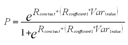 If more than one variable had been carried
forward in the original analysis, then the bracketed term would be repeated for
Var2, Var3 etc.
If more than one variable had been carried
forward in the original analysis, then the bracketed term would be repeated for
Var2, Var3 etc.
The regression constant was shown to be -1.313 and the Regression coefficient for 'smoking was shown to be 2.270....
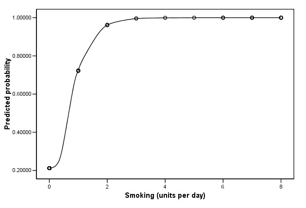
If we substitute values of 2, 3 and 4 for 'Var value1' (smoking) into the above equation you can see that as the number of smoking units increases, so does the probability of having a chesty cough.......
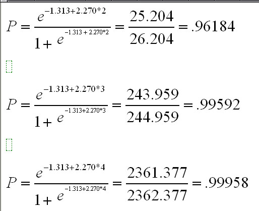
These same figures appear in column 6 of the dataset once the 'probabilities saved' facility has been used. Thus the column highlighted represents the computed probabilities of someone having a chesty cough and we know that only the smoking variable was included in the analysis
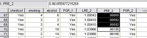
These probabilities should be plotted on a chart. Simply go to scatter graphs and place 'smoking on the X axis and PRE_2 on the Y axis......
A second example..... this time, all the variables are categorical....
 Approaching people in the street to ask them to fill in a questionnaire can be
intimidating for many people. So does it make any difference to the way people
respond to personal questions if the interviewer is male or female?
Approaching people in the street to ask them to fill in a questionnaire can be
intimidating for many people. So does it make any difference to the way people
respond to personal questions if the interviewer is male or female?
Or is the situation more complex in that people give answers that are different if being interviewed by someone of the opposite sex?
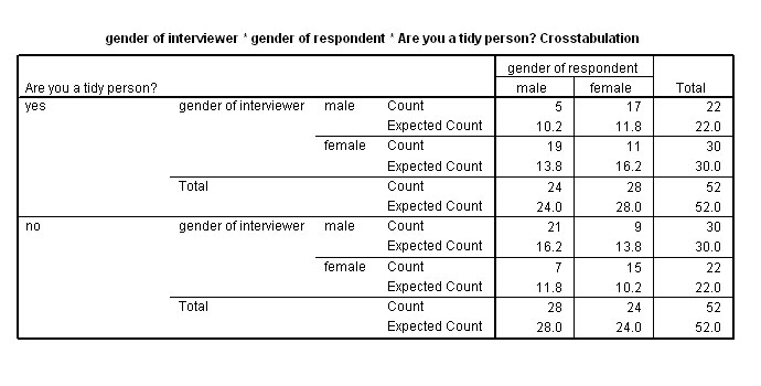
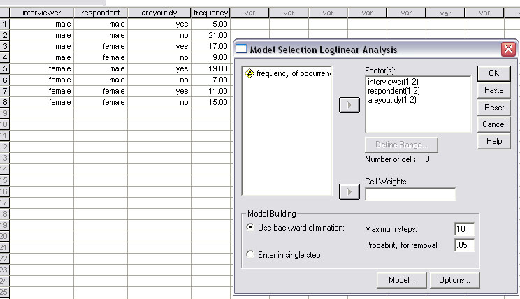
In a promotion for a new vacuum cleaner; we asked 52 females and 52 males if they considered that they kept their house tidy. Half of each group(26) were interviewed by a female and the other half by a male.
Here are the results displayed in a number of ways....
Are
you tidy at home? | Total | ||||
Interviewer | Yes | No | |||
MALE | Respondent | Male | 5 | 21 | 26 |
Female | 17 | 9 | 26 | ||
Total | 22 | 30 | 52 | ||
FEMALE | Respondent | Male | 19 | 7 | 26 |
Female | 11 | 15 | 26 | ||
Total | 30 | 22 | 52 | ||
"Do you keep your house tidy?" More females considered themselves to be tidy people than the men did.
Respondent | %
Male saying "yes" | %
Female saying "yes" | %
overall |
46.15 | 53.85 | 50.00 |
This is confirmed in the first output of the analysis....the "no regression; maximum predictability" starting point....
Overall, the male interviewers obtained more "no" responses (30) than the female interviewers did (22) and the females interviewers got more "yes" responses (30) than the male interviewers (22). So did the respective genders of the interviewer and interviewee (or the interaction between opposite sexes) make any difference to the answer given to the question? Logistic regression might give us some answers. We are interested to know if any interaction between the two categorical variables indicates that people are more likely to say that they are tidy when interviewed by someone of the opposite sex.
Use the dataset SPex 83 Interviewers
The SPSS procedure is as before except....
Transfer
the variables as indicated in the screenshot below. Then highlight the two variables
showing in the left-hand window. Use the CTrl key to do this.
The interaction
button will become operative now, so transfer Interviewer*Respondent also to the
right-hand window. This will enter the interaction possibility into the analysis
as a fresh covariate.
The 'Categorical' button will also now be active, open that window and transfer both 'Interviewer' and 'Respondent' to the Categorical Covariates box. and click 'continue'.
Under 'Options' select 'Iteration history' and under 'Save', tick 'predicted group membership' and 'probabilities'.
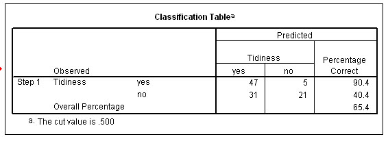
As
with the previous example, it is useful at this stage to see if the effort has
been worthwhile, have we improved the predictability of group membership by carrying
out the regression? To do this, simply compare outputs 5
& 11. The best level of predictability is now 65.4%.
An improvement
of 15.4 %
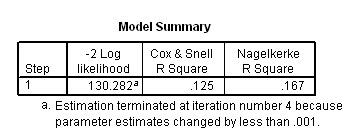
Note that the Nagelkerke R square figure for the 'goodness of fit' of the model is poor (.167) and this suggests that the model is weak and although it does improve the level of predictability, the contribution is nevertheless relatively low.....
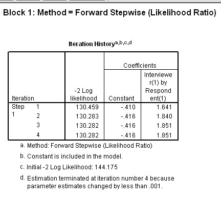
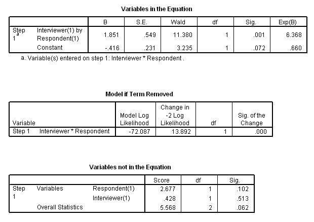
Continuing however, the next task is to determine which of the variables (and / or covariates) were utilised in the Block 1 analysis. Output 8 shows there were 4 iterations and that only the interaction covariate was entered in the final model. This means that both predictor variables were discarded.
Three further outputs help to confirm the situation. Firstly, that the only variable left in the equation is is the covariate.....and the lower charts show that if that covariate term were to be removed from the final model, it would have a highly significant effect on that model.
Our conclusions from the SPSS analysis should revolve around the fact that it was only the interaction between interviewer and respondent that produced a highly significant effect. The interpretation from that must be that people are more likely to suggest that they consider themselves tidy when being interviewed by a person of the opposite sex.
You may find it helpful to tabulate these results in a pictorial fashion....
Do you consider yourself to be tidy? | Interviewer | M | M | F | F | M | M | F | F |
| Logit residuals | -5.2 | -1.66 | -1.66 | -1.66 | 1.24 | 2.52 | 2.52 | 2.52 | |
| Observed response | Y | Y | Y | Y | N | N | N | N | |
| Respondent | M | F | F | M | M | F | F | M | |
| Prediction | N | Y | Y | Y | N | Y | Y | Y | |
| n cases (total = 104) observed | 5 | 17 | 11 | 19 | 21 | 9 | 15 | 7 | |
| n cases correctly predicted | none | 17 | 11 | 19 | 21 | none | none | none |
The situations of agreement are highlighted in blue and the situations where the prediction is the reverse of the observed values are coloured green. The total 'n cases correctly predicted' are: 68 / 104 = 65.4%
There is yet another way to assess this data...........
Loglinear analysis
 Let us rework the example above about whether people admit to being tidy or not
in an interview.
Let us rework the example above about whether people admit to being tidy or not
in an interview.
Loglinear analysis can be used to analyse multiway contingency tables such as the one in the previous example. Very precise models of the data can be achieved in this way and in particular, we can search for interactions as well as main effects. The process depends upon the frequency of occurrence of the responses and not upon mean values (as in factorial ANOVA analysis) hence categorical independent and dependent variables are fine in this context. As before, we will be testing for significance of the two independent variables and for any significant reaction between the two.
You should read the Focus page on Chi-square (Focus 8a) to understand more about contingency tables and frequency of occurrence. The process begins with what is called a 'saturated model', that is where all possible effects are included in the model-building process. Variables and /or interactions are then removed in the hierarchical order of influence (a process called 'backward elimination') until we arrive at the model that give the best 'goodness of fit'. The process continues until no improvement is recorded. This may be after 1, 2,3, or 4 iterations.
Task: Carry out a Log-Linear analysis of this data. SPex84 loglinear, interviews is available in the correct format for this analysis but it is the same dataset as before.
It is first necessary to run a 3-way crosstabs check for low expected frequencies (<5). If these occur, the analysis is unsuitable but in this instance the lowest expected frequency is 10.2.
Task: work out (using SPSS)how to do this crosstab for yourself.
So
now go to 'Analyse', 'Loglinear' and 'Model Selection'
Transfer all three variables
to the factor(s) box and define all three by their ranges (1 and 2)
Click on
'backward elimination', click 'OK'
Note that the output for this analysis
is not in the usual SPSS format
The outputs are extensive but you will note that only one iteration is made, meaning that the saturation model is also the best fit model and that the 3-way interaction cannot be eliminated. The Chi square value is 16.538 and p< .001.
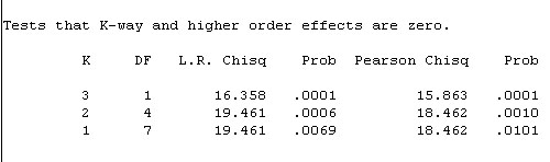 Thus none of the 3 possible 2-way interactions were significant. Our conclusion
must be that there is only a three way interaction. There is no association between
the interviewee and the answer given or between the interviewee and the answers
given but when the two are considered together they do influence the answers given.
The gender of both interviewer and respondent have a bearing on the answers given.
Thus none of the 3 possible 2-way interactions were significant. Our conclusion
must be that there is only a three way interaction. There is no association between
the interviewee and the answer given or between the interviewee and the answers
given but when the two are considered together they do influence the answers given.
The gender of both interviewer and respondent have a bearing on the answers given.
Task: Do you agree with this summary or can you place a different interpretation on the result?
![]()
Go on to Focus 18
Go back to Focus 16
Go back to 'quick view' contents