
[Focus 8a]The Chi-Square test (for Association)(and Yates' correction)A short note about 'G'-tests |
So far, we have looked at methods for determining whether or not there is a significant difference between two means using un-paired and paired t-tests and similarly; medians using Mann-Whitney / Wilcoxon tests. We have drawn a distinction between data sets that are related (interact)(matched) and those data sets that are completely independent of each other.
You may have noted that we have never tried to analyse Nominal data, the data has always been on the Ordinal, Interval or Ratio scales, so let us review what is meant by Nominal data.....
It is data that is recorded in 'name only'. It only has qualitative properties and even when numerical values are assigned according to frequency of occurrence; they have no calculable worth other than to assign each piece of data to a grouping and record the numbers in each group. Often the data represents opposites such as 'better' and 'worse'. It is this idea of 'groups or categories' that we must now use for our next analysis. Much of the Inferential statistics discussed in later Focus pages is concerned with attempting to sort large data sets into these more manageable 'categories'.
Examples of 'categories' might include:John,
Richard, Bill, David |
By recording the frequency of occurrence of the given entity / value and putting them into the correct categories, we can compare it to another frequency.
There is more; we can carry out a test to see if there is a statistically significant association existing between two variables on the Nominal scale using a Chi-square test......
The Chi-square test is similar to the parametric tests dealt with in Focus pages 4 - 8 in that:
|
The first type of Chi-square test can be used in 1-sample analysis and is often referred to as a 'goodness-of-fit' test. The second type of Chi test can be used for 2-sample and multiple sample situations and is referred to as the test for association..
Chi
tests begin with the construction of a contingency table.
This simply means a table that can be sub-divided in two directions. You will
also see the term 'cross tabulation' used, especially when using SPSS. 'Cross
tabulation' / Contingency tables are used for summarising two frequency distributions.
One variable is presented along the horizontal axis (A / B) and the other (1 /
2), along the column axis.
In its simplest form therefore.......
| 1 |
2 |
TOTAL | |
| A |
A1 |
A2 |
A1+A2 |
| B |
B1 |
B2 |
B1+B2 |
| TOTAL |
A1+B1 |
A2+B2 |
A1+A2+B1+B2 |
A basic example is shown below where 50 men and 50 women were recorded for frequency of occurrence of dark hair or fair hair colour....Remember, all columns and rows must total correctly at all times
| Dark
hair | Fair
hair | TOTAL | |
| Men |
40 |
10 |
50 |
| Women |
20 |
30 |
50 |
| TOTAL |
60 |
40 |
100 |
This format is called a 2x2 contingency table. Tables can be any size; 2x3, 3x3, 4x4 etc but 5x5 is usually as large a number of variables as would be used in this type of test.
We
will see that Chi tests are very versatile and can be readily used to investigate
a wide variety of situations but they are particularly useful in analysing a range
of questionnaire question-types where nominal data is involved. |
In this test, we only have one variable and the comparison to be made will only be against an expected occurrence for that value (E). We are testing to see if the observed values (O) are significantly different from the expected value.
"Goodness of fit" refers to the idea "how close to the expected frequencies are the observed values we obtained"? or "Do the observed values fit with the expected ones"? If there is a "good fit", it will mean there is no significant difference and we confirm the null hypothesis. If the reverse occurs and there is not a good fit between observed and expected values; then we accept the alternative hypothesis.
| Caution:
Any contingency table that includes an (E)expected value of less than 5 is unreliable. |
 Suppose we are monitoring how many underground trains are late arriving at Earl's
Court station each morning. This is the frequency of lateness of the trains but
is there any real difference between the days; there were 32 on Tuesday but only
25 on Thursday...
Suppose we are monitoring how many underground trains are late arriving at Earl's
Court station each morning. This is the frequency of lateness of the trains but
is there any real difference between the days; there were 32 on Tuesday but only
25 on Thursday...
| Day |
Late trains |
| Mon |
27 |
|
Tues |
32 |
|
Wed |
30 |
|
Thurs |
25 |
|
Fri |
27 |
|
Total |
142 |
or displayed as a bar chart.......
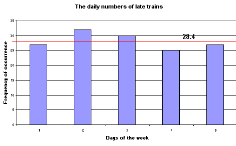
Taken over the week, there was an average of 28.4 late trains per morning. In this context we would call this our expected value (E).
They are all supposed to be carrying out exactly the same duty (viz: arriving on time) so we could propose a hypothesis:
H0 "the distribution is uniform and there is no significant difference in 'degree of lateness' between the days".
H1 "the distribution is not uniform and there is a significant difference between the days"
We will set our significance level at 5% to test whether the distribution is uniform or not.
n =5 and therefore the degrees
of freedom = (n - 1) = 4.
All you need to know to calculate the critical value are the degrees of freedom involved and your selected significance level (see Wheater and Cook, p223).
So from Chi-square tables, the critical value is, (df =4)(P 0.05) = 9.488
Since H0 propose a uniform distribution, we would expect all the operators to complete the same number of tasks within the set limits. The Chi test will 'measure' how far apart the observed values are from the expected ones.
The Expected value (E) will be 142÷5 = 28.4
The actual formula for the Chi square test looks like this:
where O is the observed values and E, the expected values.
So, to calculate out the test statistic (chi) we need to complete the following table:
| O |
E |
(O - E) |
(O - E) squared |
(O - E)squared ÷
E |
| 27 |
28.4 | -1.4 |
1.96 | 0.069 |
| 32 |
28.4 | 3.6 |
12.96 | 0.456 |
| 30 |
28.4 | 1.6 |
2.56 | 0.090 |
| 25 |
28.4 | -3.4 |
11.56 | 0.407 |
| 27 |
28.4 | -1.4 |
1.96 | 0.069 |
| Test statistic = 1.09 |
To yield a significant result, our test statistic must be higher than the critical value. In this instance; it is clearly not.
1.09 < 9.488
We must therefore confirm the null hypothesis and state that the there is no significant difference in the degree of lateness between the days. In one sense, H0 has shown itself to be independent of 'days of the week'. If we had needed to accept H1, then the conclusion would have been that there was a dependence between the 'days of the week' and the lateness of the trains.
Now let us take a second week where there were still 142 late trains but the daily
numbers were far more erratic. Is there a significant difference now between the
days?
| Day |
Late trains |
| Mon |
14 |
|
Tues |
33 |
|
Wed |
17 |
|
Thurs |
40 |
|
Fri |
38 |
|
Total |
142 |
Task: Produce a bar chart similar to the one above
| O |
E |
(O - E) |
(O - E) squared |
(O - E)squared ÷
E |
| 14 |
28.4 | -14.4 |
207.36 | 7.301 |
| 33 |
28.4 | 4.6 |
21.16 | 0.745 |
| 17 |
28.4 | -11.4 |
129.96 | 4.576 |
| 40 |
28.4 | 11.6 |
134.56 | 4.738 |
| 38 |
28.4 | 9.6
| 92.16 |
3.245 |
| Test statistic = 20.605 |
20.605 > 9.488. The result is significant, we must accept H1
From Chi-square tables, the critical value is, (df =4)(P 0.01) = 13.277
20.605 > 13.277 and so the result is also significant at the more rigorous level.
The first point to note with this test is that we are not limited to discussing only two variables (or groups) at a time. We can deal with any combination because the contingency table can be made to accommodate any number of both. Realistically however, it is unwise to construct a contingency table any bigger than 5*5 or 6*4.
| Multiple comparisons created by dealing with >2 variables is dealt with again in Focus10a (Pearson's Correlation), Focus 12 (Multiple Regression) and Focus 14 (Principal Component Analysis). |
 An international PR company encourages its staff to use the firm's indoor fitness
facilities. In order to utilise them to the optimum degree it would be a good
idea to find out which of the 3 main activities on
offer appeal to the 385 staff. There are 148 males and 237 females employed by
the firm.
An international PR company encourages its staff to use the firm's indoor fitness
facilities. In order to utilise them to the optimum degree it would be a good
idea to find out which of the 3 main activities on
offer appeal to the 385 staff. There are 148 males and 237 females employed by
the firm.
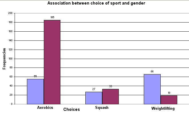
Is there a significant association between gender and choice of activity or not?
Each employee was asked to choose one of the three options. The results are given below but there are other figures in brackets....these are the expected (E) results one would obtain if there was absolutely no association between the two variables....in this case 'sport choice' and 'sex'.
Note: when the calculated EXPECTED values are low the results of a Chi test for Association become unreliable.
| Aerobic |
Squash |
Weightlifting |
totals | |
| Males |
55
(92.26) |
27
(23.06) | 66
(32.68) | 148 |
| Females |
185
(147.74) | 33
(36.94) | 19
(52.32) | 237 |
| Totals |
240 |
60 |
85 |
385 |
Row totals
are calculated and so are column totals and a grand total.
Each Expected
value(E) is now found by multiplying the row x column totals and dividing
by the grand total.
For
a 3x2 contingency table
(as above) do this 6 times...
E.g. (148 x 240) ÷ 385 = 92.26
It would appear that the women prefer Aerobics and the men prefer Weightlifting. This may be to do with childhood influences, peer pressure or a number of other possible factors. However, there were a lot fewer men in the survey to start with; so how does this affect things? Can we establish anything else from these figures?
We will be comparing the Observed values with the series of calculated (Expected) values.
Is there really an association between the sport choice and the sex of the participant?
Be very careful here....we are not trying to make comparisons between the different sports themselves but simply between 'sports choice' and sex of participants.
We begin with a null hypothesis:
" There is no association between choice of sport and gender"
These are the OBSERVED (O) values and might well be displayed as a Bar chart...
(Men = Blue bars, Women = Red bars)
The EXPECTED (E) values will reflect what we would expect to find if there were no association between sex of participant and the choice of sport. The equivalent chart looks like this....
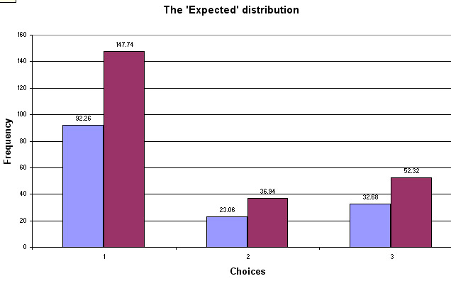
Note that expected frequencies do not have to be whole numbers but that the column and row totals must still add up to the same as for the observed frequencies. In fact, this is a useful cross check method.
The first figure of 55 gave an expected value of 92.26, because (148 x 240) ÷ 385 = 92.26 and so on for all 6 frequencies. What this means is that if there were absolutely no association between the frequency of 'sport chosen' and the gender of the participant; given the total numbers of each gender present, we should have found 92 men wanting to do aerobics rather than the 55 who actually did.
As before , we construct a table that records all the differences between the observed and expected readings...
| Observed |
Expected |
O
- E | (O
- E)squared |
(O - E) squared ÷E |
| 55 |
92.26 |
-
37.26 | 1388.31 |
15.05 |
| 185 |
147.74 |
37.26 |
1388.31 |
9.40 |
| 27 |
23.06 |
3.94 |
15.52 |
0.67 |
| 33 |
36.94 |
-
3.94 | 15.52 |
0.42 |
| 66 |
32.68 |
33.32 | 1110.22 |
33.97 |
| 19 |
52.32 |
-
33.32 | 1110.22 |
21.22 |
|
sum:
80.73 |
So our test statistic value is 80.73 and must be checked against a critical value in the tables.
We also need to know how many degrees of freedom exist and this is always "Number of rows minus one times number of columns minus one"
| Contingency
table size | degrees
of freedom |
| 2
x 2 | 1 |
| 2 x 3 (or
3 x 2) | 2 |
| 3 x 3 |
4 |
| 3 x 4 |
6 |
| 4 x 4 |
9 |
| 5 x 5 |
16 |
In this case: (2-1) x (3 -1) = 2
The tabulated value (2df) (P = 0.05) is 5.99.
The tabulated value (2df) (P = 0.01) is 9.21
The results are only significant if our calculated value exceeds the tabulated value. Our figure of 80.73 clearly does and this means that the results are significant and so we must now accept H1.
Conclusion: "There is a highly significant association between the sex of the participant and their choice of sport".
Note: We are still not in a position to define what the nature of that association might be.
Q. Go back to the bar chart; where is the most (and the least) contribution to such a strong association between the sex of the participant and the choice of sport coming from?
Compare your ideas to the figures in the right hand column above. What do you see?
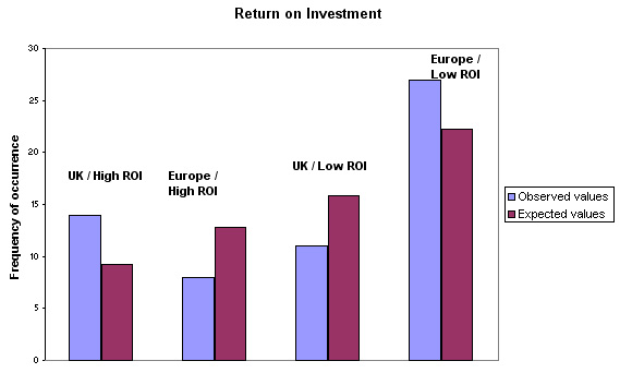
 A consumer finance magazine intends to survey 60 comparable
International manufacturing companies (25 based in the UK
and 35 from Europe) for a headline article in the next issue. The
theme of the proposed article is controversial: to highlight the differences in
Return on Investment (ROI) from UK based companies and Chinese companies. There
is not the time to carry out a detailed survey so they must dispense with the
idea of ranking each one. All they will do is mark them as 'high return' or 'low
return', hence the fact that this is still nominal data.
A consumer finance magazine intends to survey 60 comparable
International manufacturing companies (25 based in the UK
and 35 from Europe) for a headline article in the next issue. The
theme of the proposed article is controversial: to highlight the differences in
Return on Investment (ROI) from UK based companies and Chinese companies. There
is not the time to carry out a detailed survey so they must dispense with the
idea of ranking each one. All they will do is mark them as 'high return' or 'low
return', hence the fact that this is still nominal data.
We must accept right from the outset that the results will not be as robust as
they would be if a more stringent assessment were to be carried out. Note that
it is not necessary to have the same number
of cases in each row.
What question are we actually trying to answer here?.
Task: Construct H0 and H1
Here are the results displayed in a 2x2 contingency table with the (E) values shown in brackets:
| Location |
'High
ROI' | 'Low
ROI' | Totals |
| UK
companies | 14
(9.17) | 11(15.83) |
25 |
| Chinese
companies | 8(12.83) |
27(22.17) |
35 |
| Totals>> |
22 |
38 |
60 |
The (E) values would apply if there were no association between ROI and geographical location.
Remember:
"Row total times column total divided by the grand total for each observed
value
gives us the expected value".
Look at the table closely: in the UK we recorded 14 as 'High return' when we only expected to find 9 and in China we recorded 8 when we might have expected 13. So does this suggest that there is some degree of association between ROI and where the companies are actually based?
| Observed
(O) | Expected
(E) | O
- E | (O
- E) squared | (O
- E) squared ÷ Expected |
|
|
|
|
|
|
| 14 |
9.17 |
4.83 |
23.33 |
2.54 |
| 8 |
12.83 |
-4.83 |
23.33 |
1.82 |
| 11 |
15.83 |
-4.83 |
23.33 |
1.47 |
| 27 |
22.17 |
4.83 |
23.33 |
1.05 |
| 60 |
60 |
sum:
6.88 |
Our test statistic; Chi squared is 6.88
The degrees of freedom(d.f) are (2 - 1) x (2 -1) = 1
tabulated value (1d.f) is P(0.05) =3.84 and P (0.01) =6.64 Our value of 6.88 exceeds both of these values and so we accept H1 at the P(0.01) level .
This means that there is a strong association between ROI and location.
The Chi square
test has many applications but there are exceptions. One situation where it can
give
a misleading result is when a 2 x 2 contingency table is being used
as above; the test statistic can be inaccurate. The figure is too high and there
is a very real chance of making a Type 1 error. This means that there is an increased
likelihood of accepting the alternative hypothesis when in fact the null hypothesis
is true.
Yates'
correction goes some way towards redressing this anomaly.
The d.f. is still
1
The Yates' correction simply requires us to subtract 0.5 from each difference before squaring that difference.
From the UK vs China example:
| E |
[O
- E] | becomes
[O - E] - 0.5 | ....then
squared | .....then ÷ E |
| 9.17 |
4.83 |
4.33 |
18.75 |
2.04 |
| 12.83 |
-4.83 |
-4.33 |
18.75 |
1.46 |
| 15.83 |
-4.83 |
-4.33 |
18.75 |
1.18 |
| 22.17 |
4.83 |
4.33 |
18.75 |
0.85 |
| 60 | sum = 5.53 |
Sum the four results and we get a test statistic of 5.53 as opposed to 6.88.
From tables P(0.05)(1df) is 3.84 and P (0.01) is 6.64
Remember that the result is only significant if the test statistic is higher than the table value
Look at this again, if we had stayed with the Chi result we would have said that there was a significant association at the 99% level but the Yates' correction changes that and forces us to accept the null hypothesis of no association.... at this level.
| Critical value | Chi: test result | Yates' result | |
| P(0.05) | 3.84 | 6.88[accept H1] | 5.53[accept H1] |
| P(0.01) | 6.64 | 6.88[accept H1] | 5.53[accept H0] |
Task: Write a 150 words to submit to the magazine for their article?
Earlier pages have repeated the advice that when dealing with complicated data, you must try to visualise what the data is telling you. The clustered bar charts in the previous example separated (O) from (E) data but this is not necessary as the chart below illustrates....
When seeking to determine personal attitudes or to quantify a given situation, it is desirable to try and find out if the attitudes etc are derived from a common factor such as age, gender or income group for example. We can still use Nominal data, as in the next example where we discuss 'small football clubs' and 'large football clubs'
 'Soccer today' magazine contacted 155 league football clubs throughout the UK
and asked them to fill in a questionnaire about the average age of their players.
'Soccer today' magazine contacted 155 league football clubs throughout the UK
and asked them to fill in a questionnaire about the average age of their players.
Clubs have been divided into two groups based upon their turnover. Is there any association between the average age of the team and the size/wealth of the club?
Do smaller clubs have significantly more young players who then move on to bigger clubs? Do older players fall back on smaller clubs as they get towards the end of their playing careers?*
Is there an association between the age of players and size of the club?
Here are the tabulated figures:
| |
Average age of the team | |||
| Type
of Club | <
22 | 23
- 28 | >28 |
Totals |
| Large
| 18 |
51 |
16 |
85 |
|
Small |
32 |
15 |
23 |
70 |
|
Totals |
50 |
66 |
39 |
155 |
Tasks: Construct H0 and H1. There are 2 rows and 3 columns, so how many degrees of freedom are there? Construct and complete the analysis table as shown earlier.
When you have worked out all the (E)expected values; sum them to make sure that they add up to 155 also.
Find out if there is an association between the two variables using a manual method of analysis. Set your significance level firstly at 5% and then, if suitable, at 1%.
You should find that the Chi test statistic is calculated to be 23.59
Task: Write a short article for the magazine outlining your findings.
[ *Caution:You may have determined whether there is an association between the two factors or not but you cannot say how strong that association is yet or exactly where it features in the data]
 This next example also involves a typical questionnaire question and concerns
male and female choices regarding credit and debt behaviour and the use of credit
cards. A total of 1876 people aged between 20 and 50 were interviewed and one
question asked them to select which option most accurately described their action
/ behaviour.
This next example also involves a typical questionnaire question and concerns
male and female choices regarding credit and debt behaviour and the use of credit
cards. A total of 1876 people aged between 20 and 50 were interviewed and one
question asked them to select which option most accurately described their action
/ behaviour.
This is a determinant choice type of question:
| a) "I pay off my credit cards monthly whatever the outstanding balance is" b) " I pay off what I can and leave the remainder to run into the next month" c) "I only pay off the minimum and wait until I am able to pay more" |
Task: Construct another 3 x 2 Contingency table and construct H0 and H1. Set (P=0.01)
To understand the data in a contingency table ,you should construct a clustered bar chart first. The 'cluster' in this case will be 'sex' and the category axis will be 'action'.
This time, we will produce the chart in SPSS. Access the data :SPex 38 credit cards
Go to graphs, Bar....Select 'Clustered', click the radio button for 'summary of groups of cases', click 'Define'.
Transfer 'action' to the Category axis and 'Sex' to 'Define clusters'. Click 'OK'..........
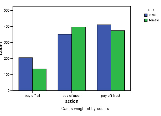
Q. Does this chart indicate the possible outcome of the analysis?
Task: Carry out a manual Chi test to see if there is any association between sex and action / behaviour . Do men and women behave differently over this issue?
The steps necessary to carry out this analysis using SPSS are describe immediately below.
Do you smoke........ and do you think smoking should be banned in pubs and restaurants?
This is called a chained
pair of dichotomous questions.
There are 4 possible outcomes:
Yes
/ Yes | Yes /
No |
No
/ Yes | No /
No |
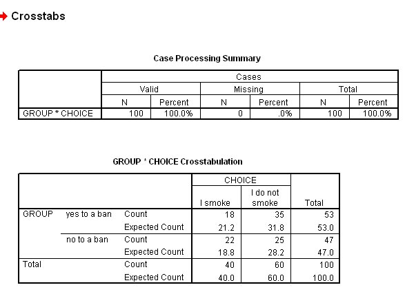
Is there any association between whether or not a person smokes and their viewpoint on a possible ban? 100 people were interviewed.
The null hypothesis says that "there is no association between the attitude people have towards a smoking ban and whether or not they smoke themselves". We are dealing with Nominal data and this is a two-group survey. With independent samples, a chi-square test of association will answer the question as to whether or not the attitudes of the two groups are significantly different.
The data can be presented as a simple 2 x 2 contingency table...
The (E) expected values (assuming no association between the factors) are shown in brackets.
'Choice'
| Ban smoking? | "Yes: I smoke" | "
No: I do not smoke" |
Totals |
| "Yes" |
18 (21.2) | 35
(31.8) | 53 |
| "No" |
22
(18.8) | 25
(28.2) | 47 |
| Totals |
40 |
60 |
100 |
Input to SPSS here is a little involved because SPSS needs to be told that these are cross tabulated frequencies (see earlier comments) and not actual values.
| SPSS Caution: in this instance, we do not use Chi from the Non-parametric menu....that is a the other Chi test, i.e, the 'goodness-of-fit' test. That type of test would be used where there was just one population e.g 40 year old men and more than two category choices such as 'walk to work', 'cycle to work', 'bus to work', 'take car to work' etc . ..... |
So: Open variable view, we need three variables. Name the variables as: 'group', 'choice' and 'count'
In the Values column (for 'group') assign 1 for 'yes to ban' and 2 for 'no to ban' and for 'choice' assign 1 for 'I smoke' and 2 for 'I do not smoke'
Switch
to data view and insert the numerical codes you have just assigned. Next insert
the values in the 'count' column
but take care to get them in the right order
and that they add up to 100!
Go to data 'drop down' menu, select 'weight cases by'. Transfer 'count' to the Frequency variable box. Click OK
Go to 'Analyse', 'Descriptive Stats', 'Crosstabs'. Transfer 'groups' to rows and 'choice' to column
Click 'Statistics' and tick the 'Chi square' box only & click 'continue'
Click 'cells' and tick both 'Observed' and 'Expected' boxes, press 'continue'
Finally click 'OK'!
This is what you should see!!
The
final part of the output will give you both the Chi test statistic and (exclusively
because this is a
2 x 2 contingency table) the Yates correction test statistic,
although you should note that SPSS calls
it the 'Continuity Correction'.
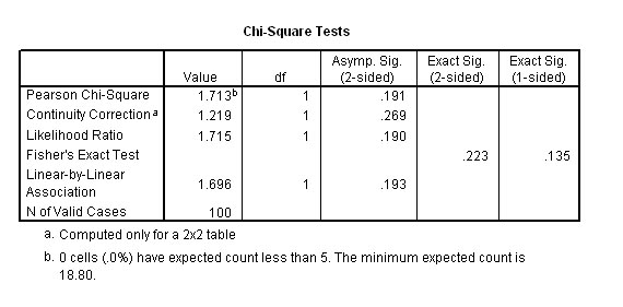
Our test statistic(Chi) is 1.713 and Yate's correction reduces it to 1.219.
The tabulated values for Chi .....(P= 0.05) (1df) 3.84.
Our
result does not exceed the critical value and is therefore not significant.
We confirm the null hypothesis
Remember when using SPSS, in the output, the P value is calculated directly. We would be looking for a value less than 0.05 to indicate a significant result. The figures to note in the above example are .191 & .269....clearly not significant.....accept H0
Note
the quite different values obtained for Chi and the correction (Yates') value
and the difference
this generates for the exact P-values.
Q. Can you comment on the risks of making a Type 1 error?.
The data set can be accessed in: SPsmex 09 Smoking ban
This time, we require a 3 x 2 Contingency table (so there are (3-1)*(2-1) = 2 degrees of freedom) and you must firstly construct H0 and H1.
 Do men and
women (aged between 30 and 60) differ in their attitudes to making a will?
Do men and
women (aged between 30 and 60) differ in their attitudes to making a will?
200 people (equal M / F) were asked to consider if the issue was: a) very important to them, b) slightly important or c) not at all important. This is a comparative rating type of question.
You can access the data: SPex 39 Making a will
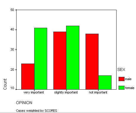
Task:Try reproducing this bar chart yourself, use SPSS....
Go to 'Graphs' in the drop down menus, select 'Clustered Bar Chart', 'Summary of groups of cases'.
The category axis will be 'opinion' and define the clusters by 'sex'
Now
carry out the analysis as before:
So:
Open variable view,
name the 3 variables as: 'sex', 'opinion' and 'scores'
In the Values column (for 'sex') assign 1 for 'yes' and 2 for 'no' and for 'choice' assign 1 for 'Very important' and 2 for 'Slightly important' and 3 for 'Not important'
Switch to data view and type in the numerical codes you have just assigned. Next insert the values in the 'scores' column but take care to get them in the right order and that they total 200!
Go to data menu, select 'weight cases by'. Transfer 'scores' to the Frequency variable box. Click 'OK'
Go to 'Analyse', 'Descriptive Stats', 'Crosstabs'. Transfer 'sex' to rows and 'opinion' to columns
Click 'Statistics' and tick the 'Chi square' box only & click 'continue'
Click 'Cells' and tick both 'Observed' and 'Expected' boxes, press 'continue'
Finally click 'OK'!
We find that the results are highly significant. The test statistic (Chi) is 13.192. The output records this highly significant result but you may wish to confirm with tables where you will find that the critical values (2df) are P (0.05) =5.991 and P(0.01) =9.210.
Remember,
a result is significant if the calculated test statistic is greater than the tabulated critical value. |
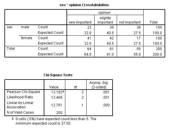
SPSS note: SPSS will not compute Chi if any of the expected counts are less than 5
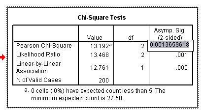
To obtain the exact level of significance; place the cursor over the .001 value and double right click and a highlighted figure will appear as shown below. This particular case shows that the true level of significance did not quite reach 0.001 but was certainly much higher than 0.01:
Summarise your findings but take care not to make deductions beyond what the Chi test results are actually telling you !
 You work for a market research company and have been assigned to lead the following
project.
You work for a market research company and have been assigned to lead the following
project.
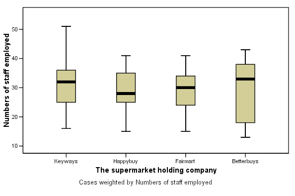
80 stores from four supermarket chains are the subject of a large survey. They are to be compared.... with respect to their staffing strategy.
The work location of 2149 staff has to be recorded. The stores are then divided into groups depending on whether they were located in Urban, Suburban or 'out-of-town' locations. Your company needs to know if there is an association between 'location' and the individual holding company with regards to staffing strategies.
All we know to begin with is that Fairmart's seem to employ slightly more staff per store than the other three chains and that suburban stores have slightly higher staffing levels than urban or out-of-town stores.
You will need to use the SPSS dataset: SPsmex 30 supermarket staff
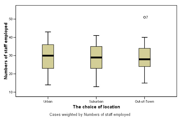
Here are the results displayed as two boxplots, firstly staff levels categorised by which holding company and then staff levels categorised by store location....
Drop
down the 'Graphs' menu and select 'Boxplots',
Select 'Simple' and 'Summaries
of groups of cases', click 'define'
Transfer 'Numbers of staff' to the 'variable box' and firstly transfer 'The supermarket holding company' to the 'Category box'. Click 'OK'. Once you have generated the boxplot, repeat but replace 'The supermarket holding company' with 'Choice of location' to generate the second plot.
The staff numbers / locations 3x4 contingency table looks like this:
Urban | Suburban | Out-of-town | Totals | |
| 'Keyways' | 78 | 58 | 154 | 290 |
| 'Happybuy' | 94 | 339 | 155 | 588 |
| 'Fairmart' | 250 | 266 | 354 | 870 |
| 'Betterbuys' | 115 | 195 | 91 | 401 |
| Totals | 537 | 858 | 754 | 2149 |
We can now carry out a Chi test for Association between Location and Supermarket group using staff numbers as the variable. Note that there is no need to know how many stores are involved or how many stores are in each location. The H0 will say that " there is no association between Location and Supermarket Group as far as staffing levels are concerned. H1 will say there is an association.
Remember first to use the 'Data' drop down menu, select 'weight cases by'. Transfer 'staffnum' to the Frequency variable box. Click 'OK'
Go to 'Analyse', 'Descriptive Stats', 'Crosstabs'. Transfer ''The supermarket holding company'' to rows and 'Choice of location' to columns. Then continue as before.......
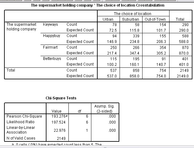
The results confirm that there is a strong association.
Task: Using tables and remembering there are (4-1)*(3-1) = 6 df. What is the critical value for P(0.01)?
Task: Write the conclusion to your findings for your line manager to read. Comment on whether you think the 4 companies are operating similar strategies or do you think that they are very different from each other?
The 'G'-test is another test of association sometimes used as an alternative to Chi. It is essentially a log linear test. There are four possible reasons for choosing this test in preference to Chi......
|
Remember, a Type 1 error occurs when we accept the alternative hypothesis when in fact we should have confirmed the null; thus concluding / stating that there is a significant relationship when there is not.
The simplest version of the test (one factor) still requires the calculation of expected frequencies for comparison against observed frequencies. Obviously in this instance we cannot look for an association when there is only one factor so it becomes a 'goodness of fit' test.
We also continue to use the Chi-square tables for finding the critical values. There is a need to look up the natural logarithm (ln) in tables of the value for 'Observed divided by Expected'. There is also a correction factor to incorporate whereby the value for G is divided by the correction factor.
In its simplest form then, the G-test is applied to a single row of data and it is here that the test is considered superior to Chi, especially (as stated) if some of the expected frequencies are low:
(where 'a' represents all the categories in the set)
 Workers from four different countries were found to be working in the administration
department of a large television broadcasting company. There is a policy of equal
opportunities operating but have the company been employing equivalent numbers
from the four countries?
Workers from four different countries were found to be working in the administration
department of a large television broadcasting company. There is a policy of equal
opportunities operating but have the company been employing equivalent numbers
from the four countries?
Our
null hypothesis will be that there is "no significant difference in the frequency
of occurrence of
staff of each nationality". The alternative hypothesis
will say that there is a significant difference.
| Nationality: |
A |
B |
C |
D |
Totals (n) |
| Observed numbers (Obs) | 24 |
32 |
10 |
9 |
75 |
| Expected numbers (Exp) | 18.75 |
18.75 |
18.75 |
18.75 |
75 |
First calculate: Ob * ln Ob ÷ E for each observation and then sum them as normal....
| 24*ln 24÷18.75 = | 5.925 |
| 32*ln 32÷18.75 = | 17.105 |
| 10*ln 10÷18.75 = | - 6.286 |
|
9*ln 9÷18.75 | - 6.606 |
| Sum (sigma) = | 10.138 |
G(initial) = 2 x 10.138 = 20.276
Next: the formula for the correction factor....
Note again that 'a' is the number of categories (i.e. 4 in this case) and that n = 75 & d.f. (n - 1) = 3
So now: 1 + (4 squared minus 1) ÷ 6* 75* 3
C.F. = 1 + (15÷1350) = 1.011
Now G(adjusted) = G(initial) ÷C.F. = 20.276 ÷ 1.011
= 20.053
Using Chi tables we find that the critical values for P(0.05)(3d.f.) = 7.815 and P(0.01)(3.d.f.) = 11.345
Hence the result is significant and we must therefore accept H1....There is a significant difference in the frequency of occurrence between the four nationalities employed by the company.
G tests can also be used as an improved alternative to Yates correction for a 2 x 2 contingency table. Unfortunately there is another complicated correction factor to be used.
However, there is no need to calculate expected values. Instead, every observed value is multiplied by the log of itself . So for example, say the value was 16 then we would calculate 16.ln16 etc. Next, these figures are all summed[A]. The same is done for the grand total [B]. Then the Row total [C] and the Column total [D] are treated in the same way.
G = 2* ([A] + [B]) - ([C] + [D])
The correction factor (Williams) is not considered here but you can see in the following example that when sample sizes are quite large, it makes little difference to the outcome of the test.
 Building Societies require their staff to be knowledgeable and courteous
to customers. The type of training they receive seems to vary considerably though.
Here is a dataset that relates to the a nationally recognised 'Welcome Customer'
training courses. 145 offices in England and Wales were surveyed.
Building Societies require their staff to be knowledgeable and courteous
to customers. The type of training they receive seems to vary considerably though.
Here is a dataset that relates to the a nationally recognised 'Welcome Customer'
training courses. 145 offices in England and Wales were surveyed.
Is there a statistically significant association between the country and whether
or not this type of course is used?
Task: Write out H0 and H1 in full
| Office Location
| Those without 'Welcome Customer' trained staff | Those with 'Welcome Customer' trained staff | Row Totals |
| England | 86 | 15 | 101 |
| Wales | 32 | 12 | 44 |
| Column Totals | 118 | 27 | Grand total: 145 |
Using the 3 test methods discussed we find that a range of test values will be generated..
The Critical value for P(0.05)(1d.f.) = 3.84
Here are the test statistic values obtained (shown from lowest to highest)..
| Yates Correction | 2.363 |
| G (corrected) | 2.896 |
| G (initial) | 2.966 |
| Chi |
3.078 |
In none of the outputs did the test statistic reach the critical value given above. Therefore in all four situations we would accept the null hypothesis. However, you can see from the 4 values that, in this instance, Yates Correction appears to be the most stringent with respect to retaining the null hypothesis and Chi the least stringent.
Perhaps this last exercise illustrates the point that there is often more than one mathematical approach to a problem and that whilst all may be valid, sometimes one method is more suited to the data than all the others.
(The G-test is not yet available in SPSS).
![]()
Back to 'Quick View' contents page
On to Focus 9