
[Focus 3 a]Histograms and SPSSand calculating the z-scores |
We have discussed the issue of using Ordinal data as though it were on the Interval scale. Such a practice can lead to serious mis-interpretation. many questionnaire designs involve some form of assigning a 'score' to a given response. For example: 1 = yes, 2 = no and 0 = don't know. Whilst the coding is perfectly valid, any numerical calculation would be meaningless...1 + 1 = 2 but "yes + yes does not equal no!"
Where 'scores' are concerned, providing the intervals are equal, it is legitimate to calculate some of the more basic descriptive outputs such as the mean and s.d. So....
 50
out of 100 first year Media students took part in a presentation skills assessment
and were graded from 1(lowest score) to 12 (highest score).
50
out of 100 first year Media students took part in a presentation skills assessment
and were graded from 1(lowest score) to 12 (highest score).
| 7 |
5 |
6 |
2 |
8 |
7 |
6 |
7 |
3 |
9 |
|
10 |
4 |
5 |
5 |
4 |
6 |
7 |
4 |
8 |
2 |
|
3 |
5 |
6 |
7 |
9 |
8 |
1 |
4 |
7 |
9 |
|
1 |
6 |
8 |
5 |
11 |
2 |
9 |
8 |
8 |
6 |
|
4 |
6 |
7 |
8 |
3 |
6 |
7 |
9 |
10 |
5 |
SPSS open program>>>what do you want to do?
Click 'type in data' (radio button)
Go to 'variable view' and give the data a proper name such as 'Prescore' [note that a maximum of 8 characters can be used].
Go to 'data view' and type in the above data.
Go to: 'Analyse', 'Descriptives , 'Descriptive Statistics'
Tick box for 'standardised values as a variable' (gives a second column with your z-values)
'Save As' requires a name and then 'Save' if you wish to keep the file.
Now open the drop down menu 'Graphs' ,'Histograms'
In the variables window that opens, transfer 'Prescore' to the right hand box using the central arrow
Tick 'display normal curve' box
Press 'OK'.
This is what you should see (using SPSS v12)....
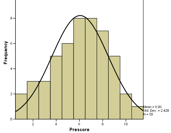
The mean, s.d and n are all displayed for you.
Q. Calculate the variance
Q. What is the z-score for a value of 2 and a value of 11?
Q. What differences might we have seen (if any) had we assessed all 100 students?
Q. Would there be any benefits from say testing 3 samples of n = 20 as opposed to 1 sample of n = 60?
A second example:
 A questionnaire team asked 100 people (at random)
whether or not they agreed that there were too many intrusive 'reality shows'
on television these days. A 1 - 5 Likert scale format was used. "No answer"
is a legitimate reponse but cannoy be used very easily in the frequency analysis.
Hence there will be a requirement to recalculate valid % reponses for all valid
responses.
A questionnaire team asked 100 people (at random)
whether or not they agreed that there were too many intrusive 'reality shows'
on television these days. A 1 - 5 Likert scale format was used. "No answer"
is a legitimate reponse but cannoy be used very easily in the frequency analysis.
Hence there will be a requirement to recalculate valid % reponses for all valid
responses.
This data is more clearly aligned to the Ordinal scale so we will confine ourselves to calculating the median and modal values and an examination of the frequency of occurrence of each possible response.
| Important! The Table layout shown below is a standard format for this type of survey and you should adopt and learn to fill out your survey forms in this fashion. |
Responses were recorded as follows:
| Value label (Likert scale) | Value | (f) | Per
cent | Cumulative
valid (f) | Valid
Per cent | Cumulative
valid % |
| No answer | 0 | 5 | 5.0 | |||
| Strongly disagree | 1 | 6 | 6.0 | 6 | 6.32 | |
| Disagree | 2 | 25 | 25.0 | 31 | 26.32 | 32.64 |
| Neither agree nor disagree | 3 | 36 | 36.0 | 67 | 37.89 | 70.53 |
| Agree | 4 | 20 | 20.0 | 87 | 21.05 | 91.58 |
| Strongly agree | 5 | 8 | 8.0 | 95 | 8.42 | 100.0 |
| Totals | 100.0 | 95.0 | 100.0 |
Your chart should look like this:
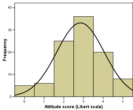
The modal value is clearly '3' :"neither agree nor disagree". The median value will be the (95 + 1) ÷ 2 = the 48th value.
The 48th value is in the cumulative (valid) class that runs from 32 to 67 inclusive i.e. Value '3' again.
A third example:
Note here that the measurement is "number of days" and as such, is legitimately on the Interval scale.
 Empire Aviation plc own 216 aeroplanes. Operational records are kept of
the number of days each plane is 'in service' each year. Listed
below are the number of days (sorted into ascending
order) that 72 of the planes (1/3rd of the fleet) were in service in 2004.
Empire Aviation plc own 216 aeroplanes. Operational records are kept of
the number of days each plane is 'in service' each year. Listed
below are the number of days (sorted into ascending
order) that 72 of the planes (1/3rd of the fleet) were in service in 2004.
| 43 |
45 |
53 |
56 |
56 |
57 |
| 58 |
66 |
67 |
73 |
74 |
79 |
| 80 |
80 |
81 |
82 |
84 |
89 |
| 97 |
99 |
100 |
102 |
102 |
104 |
| 107 |
109 |
109 |
109 |
112 |
113 |
| 114 |
115 |
115 |
116 |
118 |
121 |
| 121 |
123 |
128 |
133 |
137 |
137 |
| 137 |
138 |
139 |
139 |
145 |
146 |
| 150 |
156 |
160 |
162 |
163 |
164 |
| 174 |
178 |
179 |
184 |
186 |
191 |
| 198 |
201 |
209 |
211 |
214 |
222 |
| 234 |
240 |
249 |
251 |
266 |
270 |
SPSS open program>>>what do you want to do?
Click 'type in data' (radio button)
In 'variable view', give the data a proper name [of your choice].
Go to 'data view' and type in the above dataset in full
Go to: 'Analyse', 'Descriptives , 'Descriptive Statistics'
Tick box for 'standardised values as a variable' (z-values)
'Save' if you wish to keep the work
Go to the drop down menu; 'Graphs' ,'Histograms'
Transfer your variable to the Right-hand box as before
Tick 'display normal curve' box
Press 'OK'.
This is what you should see (here using SPSS v11)....
Large s.d's (relative to the size of the mean) indicate that there is large variation in the data, conversely, a small s.d. indicates that the data is clustered around the mean. It still always means that 68.26% of all the values will be within ± 1 s.d. of the mean. What will change is the 'peakedness of the normal distribution curve. A steep curve suggests clustering around the mean whereas a flattened curve suggests dispersion.
"Rule
of thumb": If the value of 1 s.d. is more than
a third of the value of the mean you may consider the data to be 'dispersed'. |
Q. In the above example would you say that the data was clustered or dispersed?
Task: Calculate the Variance and the s.d manually
Q.
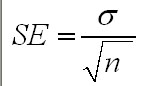
Given that we have the mean for the sample, how will this compare with the estimated
range for the mean the population ? (hint: use n-1 for a sample s.d and n for
a population). Use the 95% confidence level and the usual formula shown below.
Refer back to Focus 2a if you need help (bottom
of that page).
Q. What would happen to the difference between the s.d.values if the sample size was doubled from say 72 to 144?
Q. What would be the 'number of days' range for 68.3% of all our results?
Q. What are the z-values for the planes in service for 104, 123, and 163 days?
Q. What comments might you make about the sampling method?
![]()