
[Focus 6]The Paired 't'-test |
(a note about Standard error)
|
This is the point in the package where we embark upon inferential testing in the truest sense.
| Caution! We can only use parametric data for the tests on this Focus page. |
| There are two types: 'Paired' and 'Unpaired' (sometimes referred to as 'Matched' and 'Unmatched' and everything depends on the relationship between the two datasets. For the Paired test, we need a single group of the same subjects to be studied under two related conditions. |
We want to, in some way, quantify the difference between two samples. These samples may be people, objects, results etc but they are always going to be samples extracted from a wider population. The essential aim of this test is to assess the significance of any differences between the two sets of samples....differences between set A and set B for instance. Once we begin to think in terms of more than two sets, then t-tests are not sufficient unless a series of comparisons... A - B, A - C, B - C etc is contemplated.
The Paired (or matched) t-test is characterised by looking at the way the arithmetic means of two related sample sets behave. The greater the difference between the two means, the more likely it is that there is a real difference between the two sets.
Note however, that if the variability within the two sets is quite large to begin with( or the degree of overlap is great) then this reduces the likelihood of a real difference existing.
So we need a test that can cope with these two interlinked factors.
't' is always an index (no units) and will be the 'test statistic' we are aiming for. This idea of a test statistic was fully discussed in Focus 4. It reflects the difference between the two means (of the two sample sets) and the standard error (S.E.) of that difference. We are really calculating how many times greater than the S.E. (of the difference) the difference between the two means really is!!
Remember that the S.E. (of a mean) is the standard deviation of a set of arithmetic means from n samples. It is a measure of the average dispersion of the sample means about the population mean.
The paired 't'-test is a parametric test so we must
use data that is on the Interval or Ratio scale and normally distributed.
It
is very common in many types of enquiry / investigations to want to compare "how
things were with how they are today". Once again we are; a) making comparisons
(often over time) and
b) looking to discover if things have got better or
worse. This
t-test will test for significant differences between the means of related
groups. A single group of the same subjects is being studied under two
defined conditions. We will deal with the alternative case where the two data
sets are from different subjects in Focus 6a...the
unmatched t-test.
If
we are simply trying to establish a difference; this would require a one-tailed
test but if we want to know in which direction that difference had moved (higher
/ lower, faster / slower, better / worse etc)
we would need a two-tailed
test.
Good, rigorous procedures should try to eliminate as many misleading elements as is practicable so that we are sure that when we make a comparison.... we are comparing 'like with like'.
As
stated above, paired data means that 'pairs' of results are to be compared. It
may be a road (for accident levels at one location on two separate days) or an
individual supermarket compared over two years (for sales figures) or an Insurance
company's claims figures over a winter and a summer period. The important point
is that the subject of the two means must be the
same. Nevertheless , comparisons within paired data can
be made over time or location.
We need to more fully explain two technical terms before we can proceed....
So, S.E. (related to a mean) is the standard deviation derived from a set of arithmetic
means from n samples. It is a measure of the average dispersion of the sample
means about the population mean.....
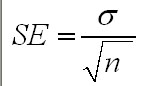
In practice, we do not need to take a large number of samples in order to calculate S.E. but instead, we can use the simplified formula shown below where we divide the standard deviation of the sample by the square root of the number of data points collected.....
 Suppose we were writing an article about acid rain caused by pollutants from power
stations. We have 25 samples of rainwater and the mean amounts of acid in those
samples was 0.8mg and the standard deviation of those samples was 0.17mg.
Suppose we were writing an article about acid rain caused by pollutants from power
stations. We have 25 samples of rainwater and the mean amounts of acid in those
samples was 0.8mg and the standard deviation of those samples was 0.17mg.
Then,
the standard error would be: 0.17 = 0.034
5
The
calculation used in the t-test follows the same logic but is slightly more involved
and the method
is best understood by a practical example:
 An Insurance Company accountant is checking the claims records. He needs to know
what the mean payout is each week over a 5 year period (260 weeks). He might decide
to check all 260 weeks but this would be unnecessarily tedious.
An Insurance Company accountant is checking the claims records. He needs to know
what the mean payout is each week over a 5 year period (260 weeks). He might decide
to check all 260 weeks but this would be unnecessarily tedious.
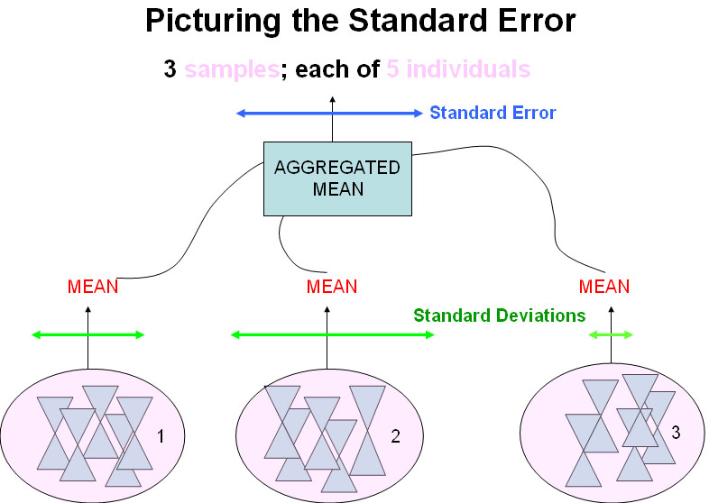
More
practically; he could check them in batches of 5 weeks and so each 5 will give
us a mean value for that period. Understandably, if we repeat the process on different
periods, we are going to get a slightly different value for the mean of each sample
of 5. However, the more we repeat the sampling, the nearer the overall mean is
going to approach the true mean for the 260 weeks. So now, instead of calculating
the standard deviation for each sample, we can calculate the S.D. for the aggregated
means that we have calculated and this is the Standard Error.
The higher the number of samples (i.e. more than 1) we choose to use, the closer we can get to a good approximation of the true mean and so the smaller the S.E. becomes.
With a t-test, we always have 2 sets (made up of pairs of data) to handle.
In nearly all inferential tests, it will be necessary to know the d.f values.
One definition is "The number of values (pieces of data) in a data set
that are free to vary".
We use d.f. of the sample (n) (as opposed to taking the full population (N)) because we need to take account of the number of independent values we have extracted or sampled from that population. By calculating any statistic (such as the mean) we inevitably loose an independent estimate of the scatter....
Suppose we weigh (n = 4) boxes (Kg):
| 80 |
140 |
| 160 |
180 |
The mean is 560 ÷ 4 = 140Kg
Now suppose we randomly pick out 3 boxes: 80, 140 and 160. The final sample has to be 180 in order that the mean should remain at 140Kg. In other words, that last sample is fixed and cannot vary.
After calculating the mean from 4 independent data points; only three will remain independent.
So: d.f. = 4 - 1 = 3
Note that where we are required to use (n - 1) that is; (population - 1 sample) the effect is going to be much greater where n is small. If n = 10 then (n - 1) will make a large difference but if n were 100 or 1000, then (n - 1) will make a very small difference. In fact, as n gets larger then (n - 1) has less effect upon the calculations and the outcome.
Hence the general philosophy in all statistics work; that you must make sure that your sample size is sufficiently large for your chosen tests to work properly. If you are faced with a very small dataset, do check carefully which tests you can legitimately use.
Note: remember that Nonparametric tests do not use absolute values but use ranks, positions etc and so n is used (where required) with no adjustments because there can be no 'mean value'.
You will also note that on your calculators, that the standard deviation of a sample is labeled as s.d (n - 1) and that of the complete population is labeled as s.d.(N)
 An advertising awareness campaign for the relaunch of a fruit-based breakfast
cereal; 'Wheetibangs' centred on the
nutritional benefits of the product.
An advertising awareness campaign for the relaunch of a fruit-based breakfast
cereal; 'Wheetibangs' centred on the
nutritional benefits of the product.
25 people were asked 15 questions
about the product before the campaign was launched and given one point for each
correct answer. The same people were asked the same questions 6 months later when
the campaign was finished. Here are the test results:

The dataset is available as: SPMe1 ad aware
Working the problem manually (n =25):Pre
Adv | Post Adv | Difference | Sum
of squared differences.... | |
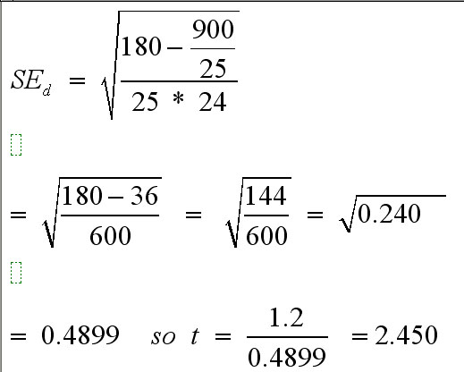
Sum | 158 | 188 | 30 | 180 |
Mean | 6.32 | 7.52 | 1.2
(d bar) | 7.2 |
The figure in blue is the mean of all the differences generated by each pair of values. This may be summarised by the first of the formulae shown below:
Next, we need to calculate the standard error of the mean difference (S.Ed.); the daunting formula above translates to:
 Correct !!
 Let us consider a busy fashion store, built in the 1970's . Head office have decided
that a complete refurbishment is required because the layout and decor is unsatisfactory,
particularly from the point of view of customer appeal. One of the post-decision
indicators that is often used in these situations is the number of customer complaints
received before and after the work
is done.
Let us consider a busy fashion store, built in the 1970's . Head office have decided
that a complete refurbishment is required because the layout and decor is unsatisfactory,
particularly from the point of view of customer appeal. One of the post-decision
indicators that is often used in these situations is the number of customer complaints
received before and after the work
is done.
Records
were kept from March to October (inc) 2003 and again from March to October 2004.
The data is 'paired' on a number of factors....same store...same months (n
= 8)......same variable .
Here are the results... (do not concern yourself with the two right-hand columns for the moment)
| Month |
Number
of complaints 2003 | Number
of complaints 2004 | difference(d) |
each
difference (d) squared |
| For SPSS>>> | compbef |
compaft | ||
| 1... Mar |
13 |
10 |
3 |
9 |
| 2... Apr |
13 |
9 |
4 |
16 |
| 3... May |
11 |
9 |
2 |
4 |
| 4... Jun |
10 |
5 |
5 |
25 |
| 5... Jul |
14 |
9 |
5 |
25 |
| 6... Aug |
12 |
8 |
4 |
16 |
| 7... Sept |
6 |
2 |
4 |
16 |
| 8... Oct |
12 |
7 |
5 |
25 |
| TOTALS |
91
(mean = 11.38) | 59
(mean = 7.38) | 32 |
136 |
Make
sure that you appreciate that the data in columns 2 & 3 is paired and must
not be separated or 'uncoupled' from each other.
The initial conclusion will
be that complaints have been reduced by:
59 ÷ 91 = 0.648 (64.8% complaints remaining). So 100% - 0.64. 8% = 35.2% reduction . This sounds impressive but is it statistically significant?
1) The null hypothesis: (be very precise) "There is no significant difference
between the mean number of complaints found before refurbishment work began and
those recorded afterwards".
The alternative hypothesis says that "there is a significant difference between the mean numbers of complaints found before refurbishment work began and those recorded afterwards".
Remember: in mathematical terms we express this as:

2) We need a two-tailed test because we want to know if the results are simply different between before commencement and after completion. The numbers of complaints might have gone up or down.
3) Carry out the test: (manually and then repeated using SPSS) always from the initial standpoint that the null hypothesis holds true:
Firstly
sum (sigma)[ ![]() ]
all the differences between the pairs......(
]
all the differences between the pairs......(![]() d
= 32), then calculate the mean difference (d bar) from:
d
= 32), then calculate the mean difference (d bar) from:
d bar = sigma d divided by n................. = 32 ÷ 8 = 4
The important formulae again:
Next, we need to calculate the standard error of the mean difference (S.Ed.) as before;
The third task is to calculate the test statistic (t): this is simply d bar divided
by the S.E:
| |
|
| t = | mean difference |
| |
S.E. of the mean difference |
So: 4 ÷ 0.378 = 10.583
Note that it is positive figure and as this is a two-tailed test the sign will tell us which direction the difference is in.
4) Compare our test statistic with the critical value from the value for 't' tables in a textbook (e.g. Curwin and Slater 5th Ed: p.635)
The degrees of freedom for a sample is always (n - 1) and so in this case it is 7(notated as 'v' in some text books)
Read off the figure for P(0.05) (df = 7) and it says 2.365. This then is the critical value for 't'.
5) Our test result (10.58) is greater than this value and so the results are significant; and so we accept the alternative hypothesis. Remember, the test statistic has to exceed the critical value for P (at the level you have set) in order to accept the alternative hypothesis.
Going back to the tables and...... reading off the value for P (0.01) (df =7), we see a figure of 3.500.
Q. What effect does this more stringent P value do to our outcome?
6) Stating our conclusion:
"
There were significantly less complaints after remedial work than there were prior
to commencement".
(t =10.58, df = 7, P < 0.05).
Q. How would you write the appropriate pair of hypotheses if you were setting the critical value at P(0.01)?
Open SPSS
Click 'enter data'
Open variable view
Name the variables as: 'compbef' and 'compaft'
Open data view
Enter the data
Go to 'Analyse', 'Compare means', 'Paired sample T-tests'
Highlight and transfer both variables to right hand box
Click 'Options', check that P is set at at 0.05 (95%).... note that you can set other levels if so desired. Under 'missing values' check that the default setting is 'Exclude cases analysis by analysis'.
Note: SPSS has the ability to deal with incomplete datasets but you have to instruct the program as to how you want that dealt with. In this instance, if one value from a pair is missing then that pair will be excluded. The alternative 'Exclude cases listwise' would mean that if a variable had even one missing value, then that would mean that the variable could not be included.
Click 'OK'
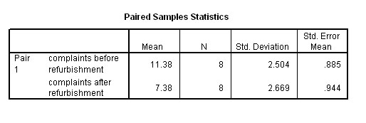
And the t-test results should look like this:
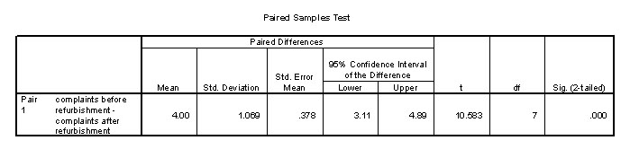
The first table tabulates the statistics for each variable. The second table in the output shows us the 't' value (10.583) and the significance as .000. This means that the result is highly significant .
| Caution: You may find that this notation is confusing but when using SPSS you must learn to recognise this format as part of the programme notation. P = 0.000 actually means "approaching 0.000", certainly P<0.0005. |
Tip: Double left click the chart and it will become hatch bordered, double left click the '.000 value' and the precise value for p will appear.....
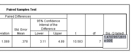
This gives an exact value for P =.000014707 and you can now appreciate that this figure is shown not to be zero. This translates to a 99.999985% Confidence Interval.
Task:
Repeat this run for yourself but using a 99% confidence interval..what happens
to the 'P' value?
Load the dataset: SPsmex
05 Store complaints
Task: Write a short summary report for the Management
Team explaining the statistical methods used and the conclusions that can be safely
drawn from the data collected. Include your justification for the use of the Paired
t-test.
 A topical newspaper investigation.....
Do 3 endorsement points on your driving licence make a significant difference to your insurance premium? Eleven companies were contacted and asked to quote for both situations (no points and three points) for the same driver and the same car. Here are the results....
| Insurance
Company | 'No
Points' Quote (£) | 'Three
Points' Quote (£) |
| A |
564 |
590 |
| B |
580 |
670 |
| C |
442 |
445 |
| D |
523 |
553 |
| E |
320 |
345 |
| F |
426 |
456 |
| G |
365 |
385 |
| H |
480 |
510 |
| I |
490 |
510 |
| J |
495 |
526 |
| K |
305 |
330 |
The null hypotheses will say " there is no significant difference between insurance quotations without endorsement points when compared to quotations involving three endorsement points". Note again that it is essential that all hypotheses are written out in full and are clear and unambiguous.
Open SPSS, 'Variable View', Name the variables as threpoi' and 'nopoi', then enter the data.
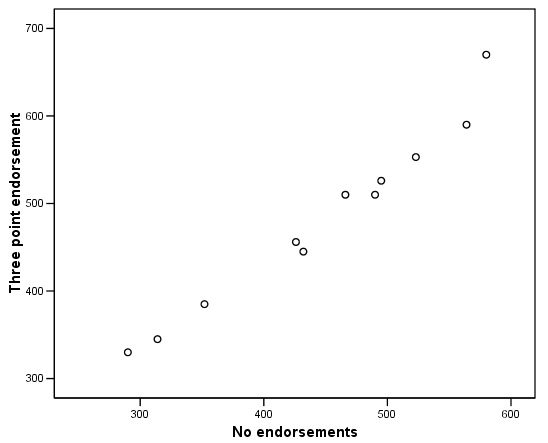
Firstly go to 'Graphs', 'scatter' , transfer the two variables to the X and Y axes. This is to check the data for anomalies before running the test.
If anomalous pairs are present you must either leave them out or consider using a non-parametric test, however, the pattern of the pairings suggest that none are present here.....
Now go to: 'Analyse', 'Compare means', 'Paired samples t-test'
Highlight the relevant pair and transfer them to the 'pairs' box. Click OK.
There are 3 tabular outputs but the third is the most important and is shown below....
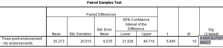
So,
the mean difference between all pairs of values is £ 35.27.
't'
is shown to be 5.845 for 10 df. The output also shows a two-tailed p-value of
0.000 but this does not signify an absolute probability and again, if you
highlight the number, the exact p-value will appear to 15 decimal places as shown
above: (0.000162750199421).
To do this;
place the cursor over the number and right click the mouse.
The 0.1% level of significance is usually sufficient for all general statistical testing. We must now accept the alternative hypothesis.
Note that our test was two-tailed, that means we were not conducting a directional hypothesis. We are only able to conclude that, "there is a significant (p<0.01) difference between the means of the two datasets and conclude that three endorsement point do make a significant difference to the insurance quotations received".
You may access this dataset at: SPsmex28 Car Quotes
 Each year the trainee management staff from 12 cinemas in the Beemax
Cinemas Group have to go through staff development training programmes
together. The pass results from 2002 and 2003 are ready for analysis. They are
normally distributed. The Regional Manager wants to know if there is a significant
difference between the results obtained in 2002 and those for 2003.
Each year the trainee management staff from 12 cinemas in the Beemax
Cinemas Group have to go through staff development training programmes
together. The pass results from 2002 and 2003 are ready for analysis. They are
normally distributed. The Regional Manager wants to know if there is a significant
difference between the results obtained in 2002 and those for 2003.
Remember: always start with a clear null hypothesis.
Load the dataset: SPsmex06 Staff Training
Task: What are the values for t and P ? Write a short report for the management team and illustrate your conclusions with a suitable comparison chart.
![]()
Go on to Focus 6a (the unpaired t-test)